Arithmetic Optimization

Usage

The Arithmetic optimization algorithm is accessible via the mealpy library using the following command:

ACTmealpy.optimize(maxiter=100, n_cpu=4, method='ArithmeticOptimization')

Example

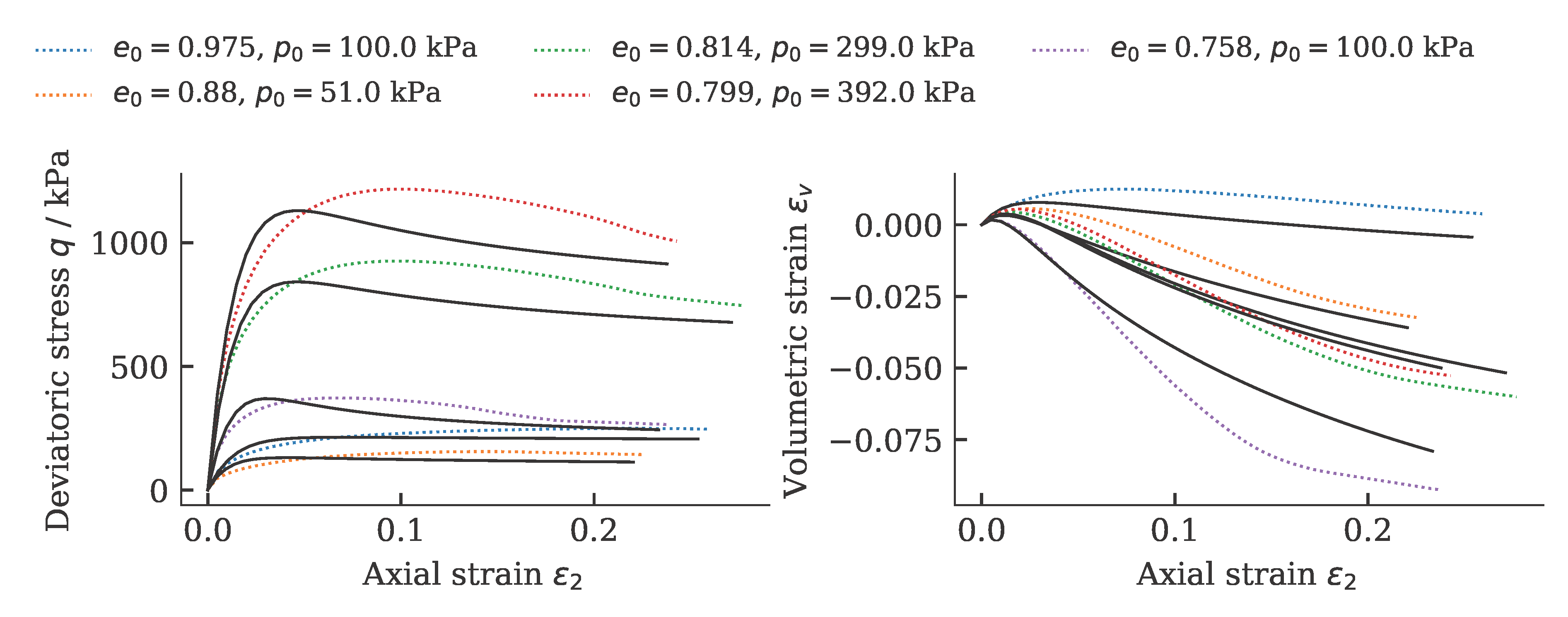
Exemplarily, the results of a calibration of a hypoplastic model ($\phi_c$, $h_s$, $n$, $e_{c0}$, $e_{d0}$, $e_{i0}$, $\alpha$, $\beta$) for Karlsruhe Fine Sand (BMU-Sand) are shown by means of drained monotonic triaxial tests:

triaxCD

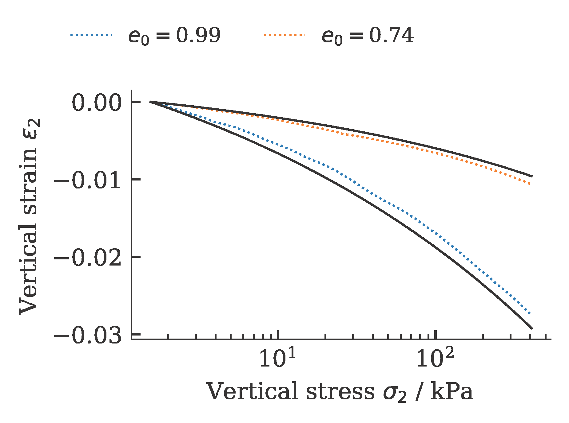
and oedometric compression tests:

oedometer

The development of the global and local cost function is shown in the figure below. It can be seen that the value of the cost function stagnates over 15 iterations. This was defined as a termination criterion for the optimization.

fitness_function

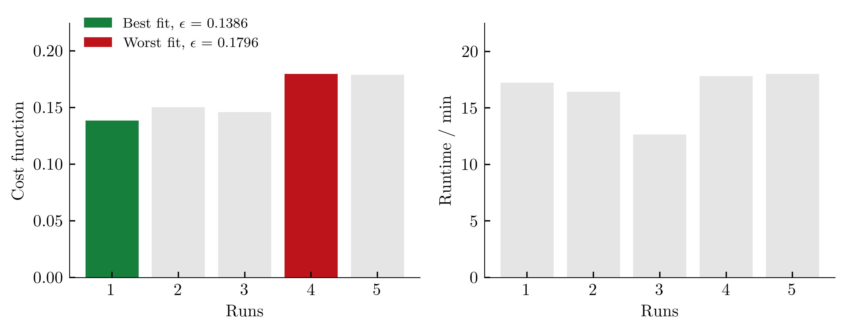
To get an (incomplete) impression about the reproducibility of the results, we repeat the calibration five times. The achieved values of the cost function as well as the required computing time per run (2x AMD Ryzen Threadripper PRO 3955WX 16-Cores, 3900 MHz, WSL2) are shown below.

statistics

The influence of the scatter in the costfunction on the simulation outcome is shown below (from large variations in cost functions, large variations in simulation results are expected):

triaxCD_all

References

[1]