Triaxial Test - Cyclic Consolidated Undrained

Table of contents

1. Finite Element (FE) representation
2. Validation of simulation approach
3. Sample numgeo input file
4. References

Finite Element (FE) representation

For the simulation of consolidated undrained (CU) cyclic triaxial tests we perform a so-called ‘‘single-element-simulation’’ with the FE program numgeo and by doing so enforce element test assumptions, i.e. a homogeneous distribution of stress/strain within the test sample. A schematic of the FE representation of the CU test is given below.

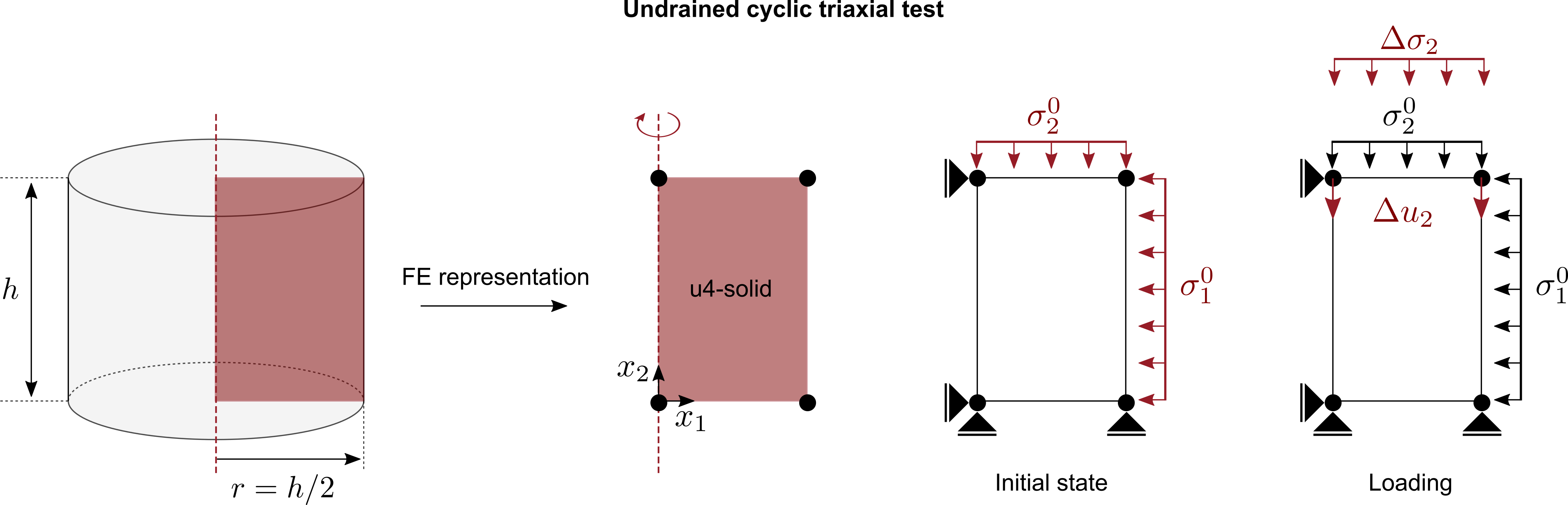
• An axisymmetric solid element with four nodes and linear shape functions for the displacement field is used. To enforce the incompressibility constrained from the undrained conditions ($tr(\dot{\boldsymbol{\varepsilon}})=0$), a locally undrained simulation is performed by assigning a Bulk modulus of pore water $K^w$. For any value of $K^w > 0$ the rate of pore water pressure is calculated as follows $\dot{p}^w = - K^w tr(\dot{\boldsymbol{\varepsilon}}) (1+e)/e$. The constitutive behaviour is governed by the effective stress $\boldsymbol{\sigma} = \boldsymbol{\sigma}^{tot}-p^w \boldsymbol{\delta}$, where $\boldsymbol{\sigma}^{tot}$ is the total stress and $\boldsymbol{\delta}$ is the Kronecker delta.
• In a first initial step, the initial conditions are applied, i.e. initial stress ($\sigma_1^0, \sigma_2^0$), initial void ratio $e_0$ or any other initial state variable required by the constitutive model to be calibrated
• In the second loading step, the loading is applied by prescribing either a periodic vertikal displacements $u_2$ of the top nodes or an additional periodic load $\Delta \sigma_2$ at the top surface of the element. The frequency of the cyclic loading is chosen as 1 Hz.

Validation of simulation approach

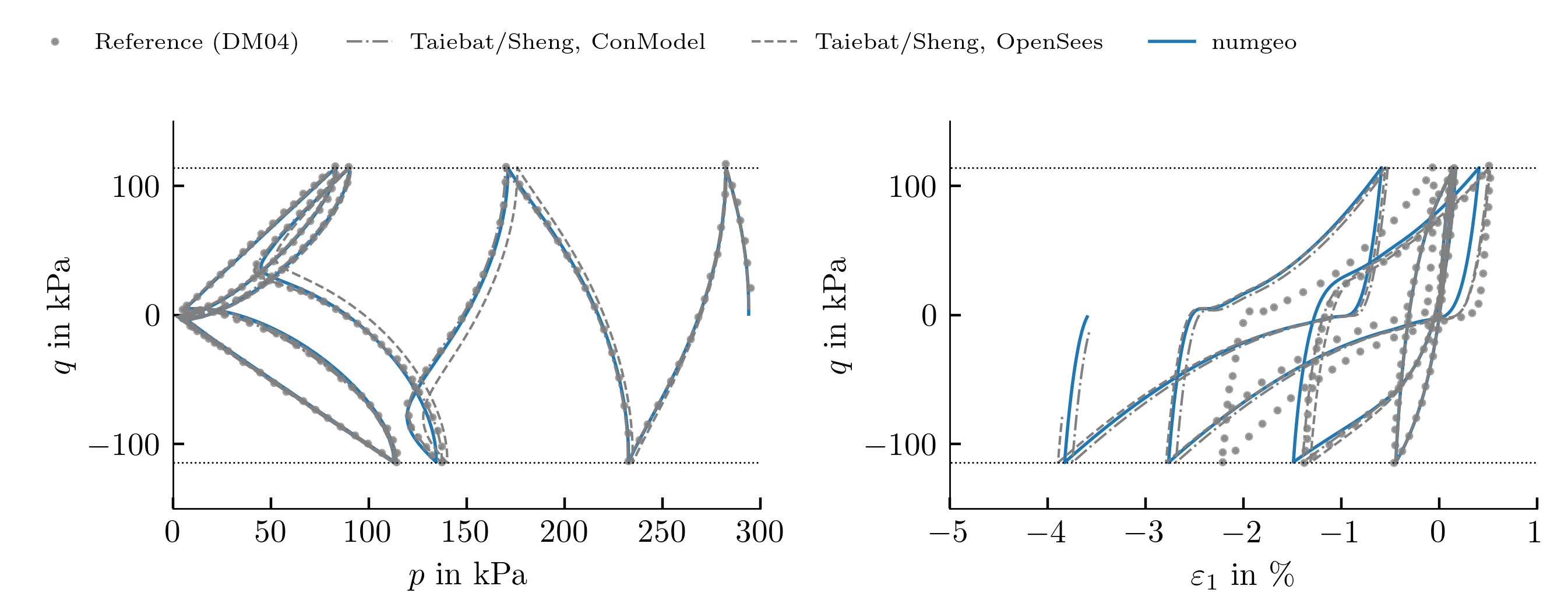
For the validation of the simulation approach, a comparison with the simulation results on Toyoura Sand with the SANISAND constitutive model reported in the original paper [1] is made. Mahdi Taiebat and Sheng Teng furthermore contributed simulation results of the same tests as in [1] such that a total of three implementations and simulation strategies could be used to benchmark the approach used in numgeo-ACT. The simulation results from Taiebat & Sheng were performed using either the finite element code OpenSees or their in-house constitutive model driver ConModel.

Sample numgeo input file

Example input file for the simulation of a stress controlled cyclic CU triaxial test using the Sanisand with numgeo are shown below.

**=~~=~~=~~=~~=~~=~~=~~=~~=~~=~~=~~=~~=~~=~~=~~=~~=~~=~~=~~=~~=~~=~~=~~=~~=~~=
**                                  numgeo                                    
**             Copyright (C) 2022 Jan Machacek, Patrick Staubach              
**=~~=~~=~~=~~=~~=~~=~~=~~=~~=~~=~~=~~=~~=~~=~~=~~=~~=~~=~~=~~=~~=~~=~~=~~=~~=

*Node
1, 0.0 , 0.00
2, 0.05, 0.00
3, 0.05, 0.1
4, 0.00, 0.10

*Nset, Nset=nall
1, 2, 3, 4, 5
*Nset, Nset=nleft
1, 4
*Nset, Nset=nright
2 , 3
*Nset, Nset=nbottom
1 , 2
*Nset, Nset=ntop
3 , 4

*Element, Type = U4-solid-ax
1, 1, 2, 3, 4

*Elset, Elset=eall
1

** ----------------------------------------

*Solid Section, elset = eall, material=soil

** ----------------------------------------

*Material, name = soil, phases = 1

*Mechanical = Sanisand-2
100,0.934,0.019,0.7,1.25,0.89,0.01,125
0.05,7.05,0.968,1.1,0.704,3.5,4,600

*Optional mechanical parameter
bulk_water, 2d6

*Density
2.65

** ----------------------------------------

*initial conditions, type=stress, geostatic
eall, 0.0, -294.0,  0.10, -294.0, 1.0, 1.0

*Initial conditions, type=state variables
eall, void_ratio, 0.808

** ----------------------------------------

*AMPLITUDE, NAME = LoadingRamp , TYPE = RAMP
0.0, 0.0, 1.0, 1.0

*AMPLITUDE, NAME = Sinus1Hz, TYPE=periodic
1,0.0,0.0,6.28
0,1

** ----------------------------------------

*STEP, name=step1, inc = 1
*GEOSTATIC

*BODY FORCE, instant
eall, GRAV, 0.0, 0, -1, 0
*DLOAD,instant
eall, P3, -294.0
*DLOAD,instant
eall, P2, -294.0

*BOUNDARY
nleft, u1, 0.0d0
nbottom, u2, 0.0d0

*END STEP

** ----------------------------------------

*STEP, name=step2, inc = 1000000, maxiter=32, miniter=1, no cutback
*Transient
0.001,4.,0.0001,0.001

*BODY FORCE, instant
eall, GRAV, 0, 0, -1, 0
*DLOAD,instant
eall, P3, -294
*DLOAD,instant
eall, P2, -294.0
*Dload, amplitude=Sinus1Hz
eall, P3, -114.2

*BOUNDARY
nleft, u1, 0.0d0
nbottom, u2, 0.0d0

*Controls, global, modify
1e-4, 5e-3, 5e-3

*output,print
*element output, elset = eall
S, E, void_ratio, fyield, flag-integration, stress-p, stress-q, stress-pw

*END STEP

*END INPUT

References

[1] Y. F. Dafalias and M. T. Manzari, ‘Simple plasticity sand model accounting for fabric change effects’, Journal of Engineering mechanics, vol. 130, no. 6, pp. 622–634, 2004.