Triaxial Test - Consolidated Undrained
Table of contents
- Finite Element (FE) representation
- Validation of simulation approach
- Sample numgeo input file
- References
Finite Element (FE) representation
For the simulation of consolidated undrained (CU) monotonic triaxial tests we perform a so-called ‘‘single-element-simulation’’ with the FE program numgeo and by doing so enforce element test assumptions, i.e. a homogeneous distribution of stress/strain within the test sample. A schematic of the FE representation of the CU test is given below.
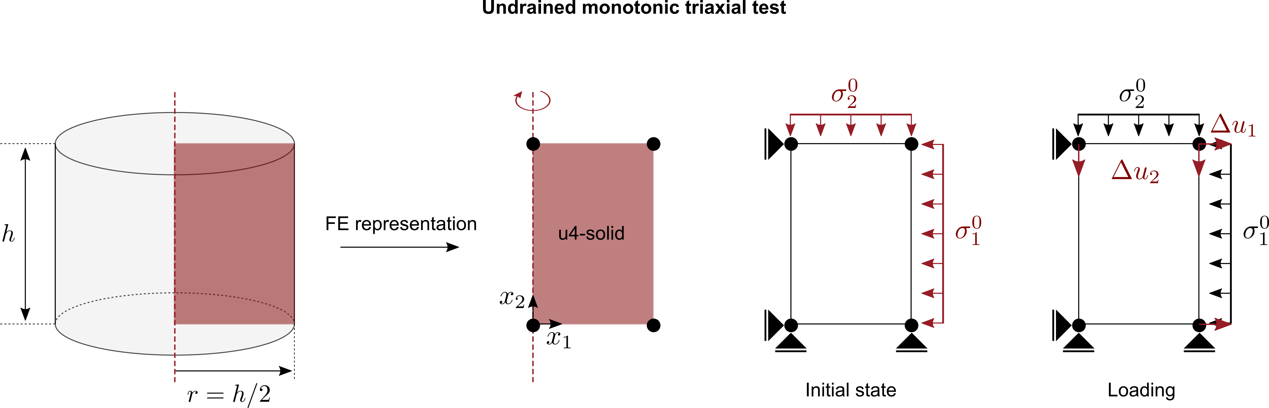
- An axisymmetric solid element with four nodes and linear shape functions for the displacement field is used
- In a first initial step, the initial conditions are applied, i.e. initial stress ($\sigma_1^0, \sigma_2^0$), initial void ratio $e_0$ or any other initial state variable required by the constitutive model to be calibrated
- In the second loading step, the loading is applied by prescribing the vertikal displacements $u_2$ of the top nodes and the horizontal displacements $u_1$ of the nodes on the right hand side of the and thus controlling the axial (vertical) and radial (horizontal) strain in the soil, respectively.
- $u_2$ is increased linearly starting from $u_2=0$ until $u_2^{max} = h \cdot \varepsilon_{lab}^{max}$ is reached. Therein, $h$ is the soil sample and $\varepsilon_{lab}^{max}$ is the maximum axial strain measured in the laboratory experiment.
- $u_1$ is controlled such that the volume of the element (sample) remains constant ($\text{tr}(\Delta \boldsymbol{\varepsilon})=0$) and thus imitating the role of pore water in undrained triaxial tests. With the present geometry of the element ($r=h/2$) this yields $u_1 = -u_2/4$.
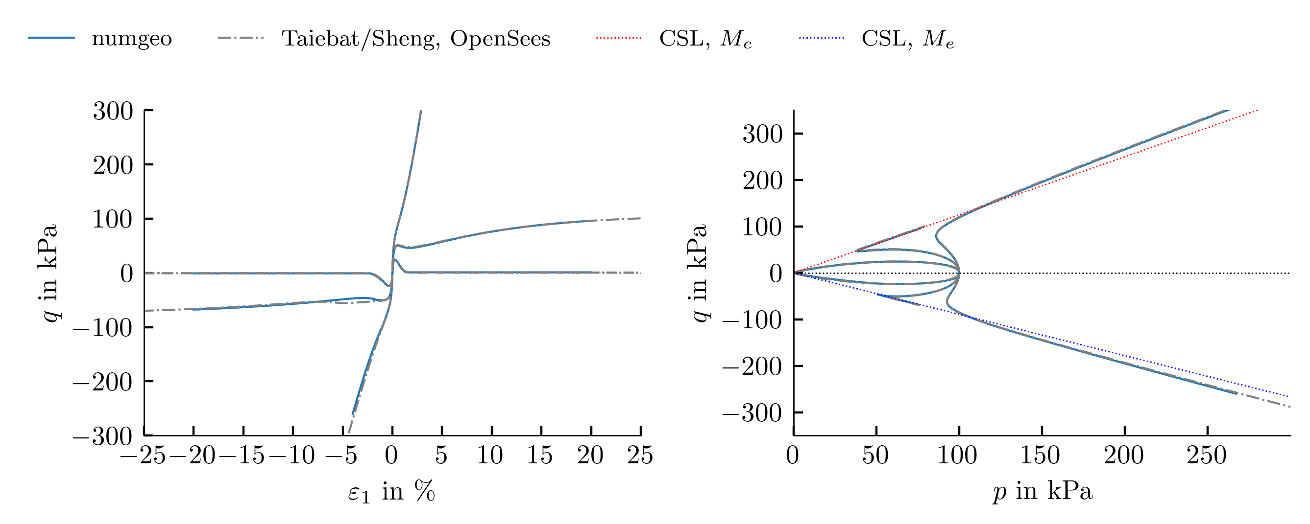
Validation of simulation approach
For the validation of the simulation approach, a comparison with the simulation results on Toyoura Sand with the SANISAND constitutive model provided by Mahdi Taiebat and Sheng Teng such that a total of two implementations and simulation strategies could be used to benchmark the approach used in numgeo-ACT. The simulation results from Taiebat & Sheng were performed using either the finite element code OpenSees or their in-house constitutive model driver ConModel.
Sample numgeo input file
Example input file for the simulation of a CU triaxial test using the Sanisand with numgeo are shown below.
Triaxial compression
**=~~=~~=~~=~~=~~=~~=~~=~~=~~=~~=~~=~~=~~=~~=~~=~~=~~=~~=~~=~~=~~=~~=~~=~~=~~=
**                                  numgeo
**             Copyright (C) 2022 Jan Machacek, Patrick Staubach
**=~~=~~=~~=~~=~~=~~=~~=~~=~~=~~=~~=~~=~~=~~=~~=~~=~~=~~=~~=~~=~~=~~=~~=~~=~~=

*Node
1, 0.0 , 0.00
2, 0.05, 0.00
3, 0.05, 0.1
4, 0.00, 0.10

*Nset, Nset=nall
1, 1, 2, 3, 4
*Nset, Nset=nleft
1, 4
*Nset, Nset=nright
2 , 3
*Nset, Nset=nbottom
1 , 2
*Nset, Nset=ntop
3 , 4

*Element, Type = U4-solid-ax
1, 1, 2, 3, 4

*Elset, Elset=eall
1

** ----------------------------------------

*Solid Section, elset = eall, material=soil

** ----------------------------------------

*Material, name = soil, phases = 1

*Mechanical = Sanisand-2
100,0.934,0.019,0.7,1.25,0.89,0.01,125
0.05,7.05,0.968,1.1,0.704,3.5,4,600

*Density
2.65

** ----------------------------------------

*Initial conditions, type=stress, geostatic
eall, 0.0, -100, 0.1, -100, 1., 1.

*Initial conditions, type=state variables
eall, void_ratio, 0.996

** ----------------------------------------

*Amplitude, name=LoadingRamp, type=ramp
0.0, 0.0, 1.0, 1.0

** ----------------------------------------

*Step, name=Geostatic, inc=1
*Geostatic
*Body force, instant
eall, GRAV, 0, 0, -1, 0
*Dload, instant
eall, p3, -100
*Dload, instant
eall, p2, -100
*Boundary
nleft, u1, 0.
nbottom, u2, 0.
*Output, print
*Element output, elset=eall
S, E, void_ratio, fyield, flag-integration, stress-p, stress-q, stress-pw
*End Step

** ----------------------------------------

*Step, name=Loading, inc=10000, maxiter=32, miniter=2
*Static
0.0005, 1, 0.0005, 0.0005

*Body force, instant
eall, GRAV, 0, 0, -1, 0
*Dload, instant
eall, p3, -100
*Dload, instant
eall, p2, -100

*Boundary, amplitude = LoadingRamp
ntop, u2, -0.02
nright, u1, 0.005

*Boundary
nleft, u1, 0.
nbottom, u2, 0.

*Output, print
*Element output, elset=eall
S, E, void_ratio, fyield, flag-integration, stress-p, stress-q, stress-pw

*End Step

** ----------------------------------------

*End Input
Triaxial extension
**=~~=~~=~~=~~=~~=~~=~~=~~=~~=~~=~~=~~=~~=~~=~~=~~=~~=~~=~~=~~=~~=~~=~~=~~=~~=
**                                  numgeo
**             Copyright (C) 2022 Jan Machacek, Patrick Staubach
**=~~=~~=~~=~~=~~=~~=~~=~~=~~=~~=~~=~~=~~=~~=~~=~~=~~=~~=~~=~~=~~=~~=~~=~~=~~=

*Node
1, 0.0 , 0.00
2, 0.05, 0.00
3, 0.05, 0.1
4, 0.00, 0.10

*Nset, Nset=nall
1, 2, 3, 4, 5
*Nset, Nset=nleft
1, 4
*Nset, Nset=nright
2 , 3
*Nset, Nset=nbottom
1 , 2
*Nset, Nset=ntop
3 , 4

*Element, Type = U4-solid-ax
1, 1, 2, 3, 4

*Elset, Elset=eall
1

** ----------------------------------------

*Solid Section, elset = eall, material=soil

** ----------------------------------------

*Material, name = soil, phases = 1

*Mechanical = Sanisand-2
100,0.934,0.019,0.7,1.25,0.89,0.01,125
0.05,7.05,0.968,1.1,0.704,3.5,4,600

*Density
2.65

** ----------------------------------------

*Initial conditions, type=stress, geostatic
eall, 0.0, -100, 0.1, -100, 1., 1.

*Initial conditions, type=state variables
eall, void_ratio, 0.831

** ----------------------------------------

*Amplitude, name=LoadingRamp, type=ramp
0.0, 0.0, 1.0, 1.0

** ----------------------------------------

*Step, name=Geostatic, inc=1
*Geostatic
*Body force, instant
eall, GRAV, 0, 0, -1, 0
*Dload, instant
eall, p3, -100
*Dload, instant
eall, p2, -100
*Boundary
nleft, u1, 0.
nbottom, u2, 0.
*Output, print
*Element output, elset=eall
S, E, void_ratio, fyield, flag-integration, stress-p, stress-q, stress-pw
*End Step

** ----------------------------------------

*Step, name=Loading, inc=10000, maxiter=32, miniter=2
*Static
0.0005, 1, 0.0005, 0.0005

*Body force, instant
eall, GRAV, 0, 0, -1, 0
*Dload, instant
eall, p3, -100
*Dload, instant
eall, p2, -100

*Boundary, amplitude = LoadingRamp
ntop, u2, 0.02
nright, u1, -0.005

*Boundary
nleft, u1, 0.
nbottom, u2, 0.

*Output, print
*Element output, elset=eall
S, E, void_ratio, fyield, flag-integration, stress-p, stress-q, stress-pw

*End Step

** ----------------------------------------

*End Input
References
[1] Y. F. Dafalias and M. T. Manzari, ‘Simple plasticity sand model accounting for fabric change effects’, Journal of Engineering mechanics, vol. 130, no. 6, pp. 622–634, 2004.