Oedometric compression test¶

In an oedometer (one-dimensional compression) test the specimen is loaded axially while lateral strain is prevented by a rigid ring. The result is a relationship between the applied vertical stress and the vertical (= volumetric) strain, from which the confined compressibility of the soil is obtained.

What it constrains¶

Oedometer tests are the primary monotonic constraint on a model's compression behaviour: how stiffness evolves with stress level and density. For the hypoplastic and ISA-type models they strongly influence the granulate hardness hs and the exponent n; for the SANISAND family they inform the compression law and the limiting void ratios.

How numgeo-ACT simulates it¶

numgeo reproduces the oedometer as a single axisymmetric finite element (U4-solid-ax) representing a cylindrical specimen of radius \(r\) and height \(h\). In the FE model the directions are \(x_1\) (radial) and \(x_2\) (axial).

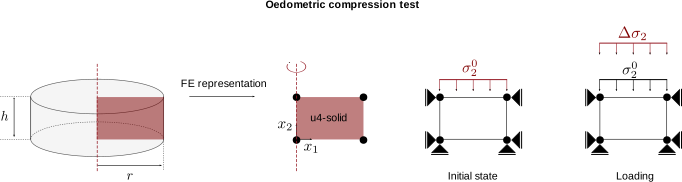
Oedometric compression test modelled in numgeo — Oedometric compression: a single-element, laterally constrained simulation. An initial axial stress is applied, then increased stress-controlled, while the radial strain is kept at zero.

The conditions under which the test is simulated are:

Lateral confinement (the oedometric condition): the radial displacement is fixed on both the symmetry axis and the outer radius (u₁ = 0 on nleft and nright), so the specimen cannot deform laterally — the only deformation is vertical, and the axial strain equals the volumetric strain.
Base: the vertical displacement is fixed at the bottom (u₂ = 0 on nbottom).
Consolidation: the recorded initial axial stress is applied to the top face in a geostatic step, starting from the initial void ratio \(e_0\).
Loading: the axial stress is increased stress-controlled to each level present in your data; the resulting axial (= volumetric) strain is what numgeo-ACT compares against your measurements.
Drainage: the specimen is dry/drained (a solid element carrying effective stresses), as in a standard oedometer.

numgeo element test

For the full numgeo input and a step-by-step description of this element test, see the numgeo tutorial Oedometric compression test.

Data mapping (`OED-#` sheet)¶

Cell / column	Meaning	Units
`B1`	initial void ratio \(e_0\)	–
row 2	column headers (informational)	–
column 0 (from row 3)	vertical stress	kPa
column 1 (from row 3)	vertical strain \(\Delta h/h_0\) (as a fraction, not %)	–
column 2 (optional)	initial-state string(s)	–

Strain is a fraction here

Unlike the triaxial sheets (which use percent), the oedometer strain column is read as a fraction — e.g. enter 0.0235 for 2.35 %.

Very small stresses are ignored

Rows with a stress below 1 kPa are skipped by the reader, so a leading near-zero seating point does not affect the simulation.

The complete cell-by-cell specification, including the optional initial-state column, is given on the Excel sheet reference. A ready-to-fill OED-1 sheet is included in the template.

Loading-unloading-reloading paths¶

An OED-# sheet may contain a full stress-controlled loading-unloading-reloading history. In that case, the order of the rows is part of the experiment and must not be sorted by stress. The same vertical stress can occur several times, but with different strains because the specimen is on a different branch of the load history.

For such data, numgeo-ACT automatically writes the oedometer simulation with a tabular stress amplitude. The complete stress history from the Excel sheet is therefore imposed on the single-element oedometer model. This is required when small-strain extensions such as IGS or ISA are calibrated from unloading and reloading loops.

Do not pre-sort LUR oedometer data

Keep the measured rows in the experimental order. Sorting the sheet by stress destroys the load history and removes the information needed to calibrate unloading/reloading stiffness and small-strain memory parameters.