Undrained cyclic triaxial test
In an undrained cyclic triaxial test the consolidated specimen is subjected to a cyclic deviatoric load with drainage prevented. Excess pore pressure builds up cycle by cycle, the effective stresses migrate towards the origin, and the specimen may reach cyclic mobility or liquefaction. This test is the key constraint on a model's cyclic, liquefaction-relevant behaviour.
What it constrains
Undrained cyclic triaxial tests constrain pore-pressure accumulation and cyclic mobility: how fast the effective stress path moves towards failure under repeated loading, and how the stress–strain loops evolve. They are essential for calibrating models used in earthquake and liquefaction analyses (e.g. the SANISAND family).
How numgeo-ACT simulates it
numgeo reproduces the undrained cyclic triaxial test as a single axisymmetric
finite element (U4-solid-ax) with \(r = h/2\), using the same constant-volume
kinematic constraint as the monotonic undrained test: the radial displacement
is tied to the axial one so the volume stays constant (undrained) throughout
cycling. In the FE model \(x_1\) is radial and \(x_2\) axial.
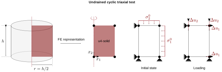
The conditions under which the test is simulated are:
- Symmetry / consolidation: as for the monotonic undrained test,
u₁ = 0on the axis,u₂ = 0at the base; the cell stress and axial stress are applied in a geostatic step. - Constant-volume (undrained) condition: enforced kinematically by linking the radial displacement to the axial displacement (\(\Delta u_1 = -\tfrac{r}{2h}\,\Delta u_2\)), so \(\mathrm{d}\varepsilon_v = 0\). The pore-fluid bulk modulus is removed from the material.
- Cyclic loading: applied under that constraint, either stress-controlled (a loading-signal amplitude drives the axial stress and the radial increment follows with the constant-volume factor) or strain-controlled (a prescribed zig-zag axial-displacement amplitude). The stress amplitude and the number of cycles \(N_\text{sim}\) come from the sheet.
Early termination at ±20 % axial strain
Some constitutive models develop excessive, runaway strains once
liquefaction is reached. Integrating such states becomes very slow, yet the
response is unphysical and does not contribute to the calibration. It would
only inflate the run time. To prevent this, the undrained cyclic triaxial
simulation carries an early-termination criterion: numgeo stops the
simulation automatically as soon as the axial strain reaches ±20 %
(a *Termination condition on the axial strain e22 at ±0.2). A run that
is terminated this way before the compared number of cycles
(Ncompare = min(Nexp, Nsim)) is treated like an incomplete simulation and
receives the penalty; the comparison itself always covers exactly the first
Ncompare cycles of experiment and simulation. The run simply does not
waste time integrating the post-liquefaction runaway. This works alongside
the per-cycle and total timeouts.
numgeo element test
For the full numgeo input and a step-by-step description, see the numgeo tutorial Undrained cyclic triaxial test.
Data mapping (CUCYC-# sheet)
Cyclic sheets carry more header information than monotonic ones: the loading amplitude, the consolidation stresses, the pore-fluid bulk stiffness and the number of cycles, followed by the recorded cyclic response.
| Cell | Meaning | Units |
|---|---|---|
B1 |
initial void ratio \(e_0\) | – |
C1 |
test name (informational) | – |
B2 |
deviatoric stress amplitude | kPa |
B3 |
consolidation axial stress \(\sigma_1\) | kPa |
B4 |
consolidation cell stress \(\sigma_3\) | kPa |
B5 |
pore-fluid bulk modulus \(K_w\) | kPa |
B6 |
number of cycles to simulate \(N_\text{sim}\) | – |
| Column (from the data row) | Meaning | Units |
|---|---|---|
| column 0 | mean effective stress \(p\) | kPa |
| column 1 | deviatoric stress \(q\) | kPa |
| column 2 | axial strain \(\varepsilon_1\) (in %) | % |
| column 3 | excess pore pressure \(p_w\) | kPa |
| column 4 | cycle number \(N\) | – |
| column 12 (optional) | initial-state string(s) | – |
Header block and data block are separated
On the cyclic sheet the header parameters occupy the first rows; the recorded cyclic data begins further down (after a spacer region). The exact starting row and the optional initial-state column are documented on the Excel sheet reference.
A CUCYC-1 example sheet with a filled header block and example data is
included in the template. The example
database database-kfs-monotonic-cyclic.xlsx contains six such tests
(CUCYC-1 … CUCYC-6).