Triaxial Test - Cyclic Consolidated Undrained

Finite Element (FE) representation

For the simulation of consolidated undrained (CU) cyclic triaxial tests we perform a so-called ''single-element-simulation'' and by doing so enforce element test assumptions, i.e. a homogeneous distribution of stress/strain within the test sample. A schematic of the FE representation of the CU test is given below.

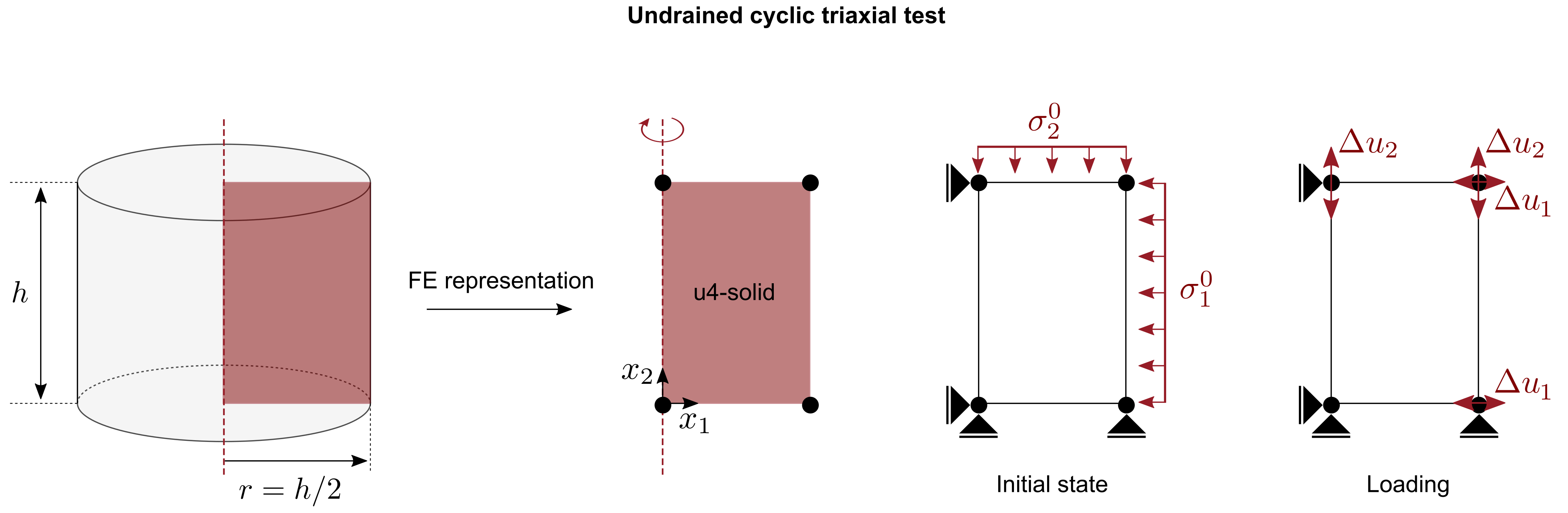
Figure 1. Single-element representation of a undrained cyclic triaxial test

• An axisymmetric solid element with four nodes, linear shape functions for the displacement field and reduced integration is used. To enforce the incompressibility constrained from the undrained conditions (\(tr(\dot{\boldsymbol{\varepsilon}})=0\)), a locally undrained simulation is performed. This can be done by controlling both the vertical as well as the horizontal displacement enforcing \(\dot{\varepsilon}_v = 0\). Some constitutive models also allow to calculate the development of excess pore water pressure in the constitutive model itself based on a prescribed bulk modulus of the pore water. The latter option has the advantage that a slight compressibility of the pore water due to minor air inclusions can be considered.
• Initial stress (\(\sigma_1^0, \sigma_2^0\)) and initial void ratio \(e_0\) or any other initial state variable required by the constitutive model to be calibrated are assigned using *Initial conditions
• The simulation starts with the loading step. The loading is applied using a special amplitude type called lab-cyclic-stress-strain-control, see reference manual for more information.

Validation of simulation approach

For the validation of the simulation approach, a comparison with the simulation results on Karlsruhe Fine Sand with the Hypo+ISA constitutive model is made.

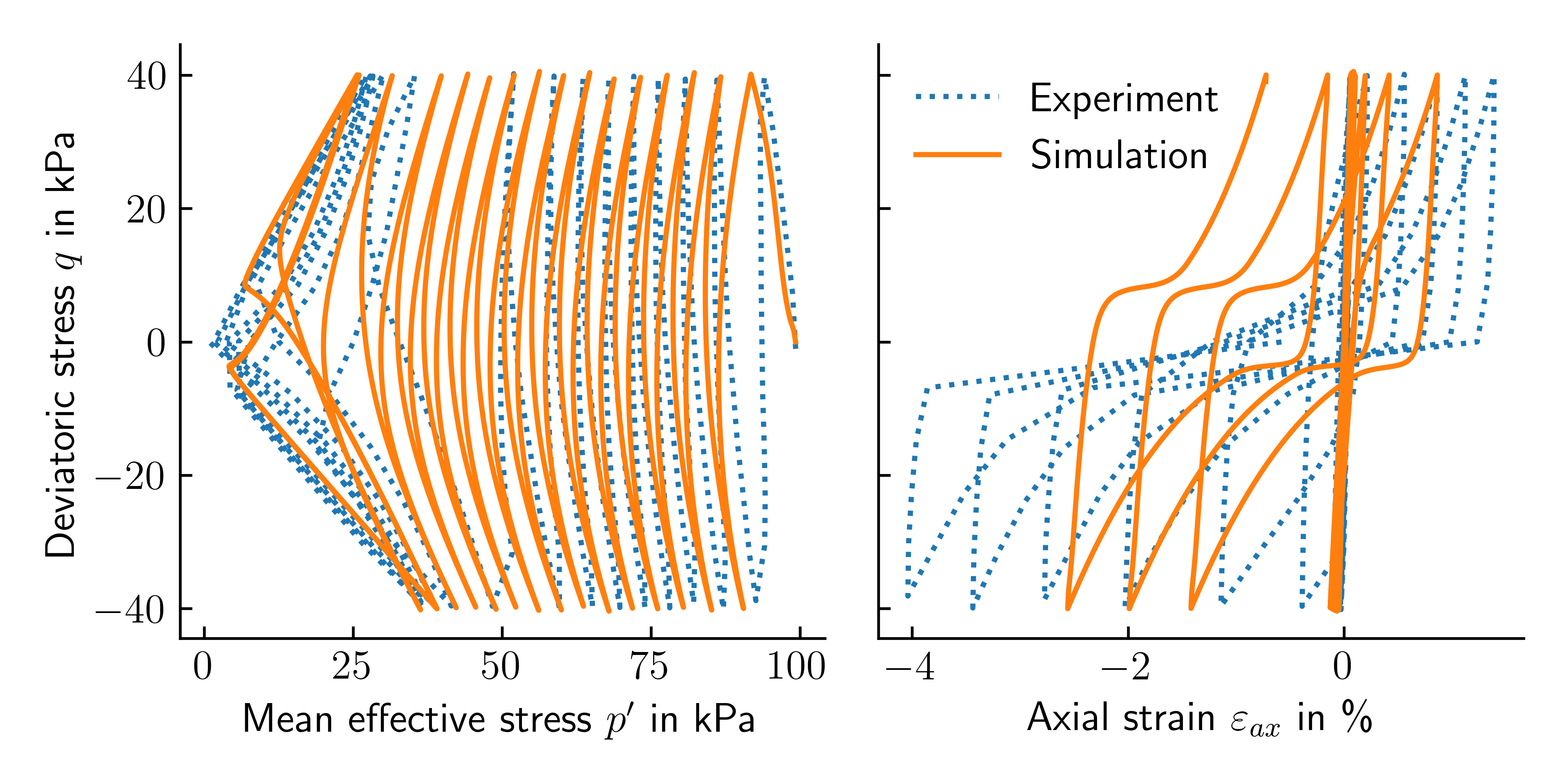
Figure 2. Undrained cyclic triaxial test on Karlsruhe Fine Sand: experiment vs. simulation

Sample numgeo input file

• First we create the four nodes defining the finite element:

  *Node
  1, 0.0, 0.00
  2, 1.0, 0.00
  3, 1.0, 1.0
  4, 0.0, 1.0
  

• We use an axisymmetric four node solid element with reduced integration (only one phase considered)

  *Element, Type = U4-solid-ax-red
  1, 1, 2, 3, 4
  

• Next, we define some node and element sets for the assignment of boundary conditions, loads and material parameters:

  *Nset, Nset = nall
  1, 2, 3, 4
  *Nset, Nset = nleft
  1, 4
  *Nset, Nset = nright
  2, 3
  *Nset, Nset = nbottom
  1, 2
  *Nset, Nset = ntop
  3, 4
  *Elset, Elset=eall
  1
  

• In order to assign the material to the element, we first create a solid section. The material name linked to this solid section is arbitrary but must be specified in a later step.

  *Solid Section, elset = eall, material = soil
  

• Define the material:

  *Material, name = soil, phases = 1
  
  *Mechanical = Hypo-ISA
  0.578,9958000.0,0.252,0.643,1.066,1.119,0.155,2.906
  1.345,0.000179,0.07,10.149,10.832,0.017,762.0,2.078
  50,0.45,1,5.0d5,1
  
  *Density
  1.8
  

  In the present example, the undrained conditions are enforced calculating the development of excess pore water pressure inside the (mechanical) constitutive model. For this the bulk modulus of the pore water is set to \(K^w=500\) MPa (4th entry in the third row).

  Note that in the present case no Hourglass stiffness needs to be added since the displacement at all nodes of the finite element are prescribed and no Hourglass modes can develop.

• Define the initial conditions of the simulation. In the present case this comprises the definition of the initial (effective) stresses as well as the initial void ratio. The initial stresses will be mandatory in most simulations that you will perform using numgeo. The initial void ratio however is only required for constitutive models incorporating the void ratio as a state variable.

  The initial stress is prescribed in terms of the initial effective vertical (or axial) stress \(\sigma_{v0}^\prime\) at two heights of the model and the initial stress ratio \(\sigma_{h0}^\prime/\sigma_{v0}^\prime\) where \(\sigma_{h0}^\prime\) is the horizontal effective stress. In the present example isotropic conditions are assumed.

  *Initial conditions, type = stress, geostatic
  eall, 0.0, -99.3, 0.1, -99.3, 1.0, 1.0
  

  Different constitutive models might require different (internal) state variables to be initialised. For the Hypo+ISA model, initialisation of the void ratio \(e_0\), the intergranular strain tensor \boldsymbol{h}$ and the intergranular back strain tensor \(\boldsymbol{c}\) is required. The intergranular (back) strain is assumed to be isotropically fully mobilised.

  *Initial conditions, type = state variables
  eall, void_ratio, 0.761
  eall, int_strain11, -0.0001035
  eall, int_strain22, -0.0001035
  eall, int_strain33, -0.0001035
  eall, int_back_strain11, -5.18e-05
  eall, int_back_strain22, -5.18e-05
  eall, int_back_strain33, -5.18e-05
  

• Next, we define an amplitude for the cyclic loading. For this we use an amplitude of type lab-cyclic-stress-strain-control. An amplitude specially designed for cyclic triaxial tests, details are given in *Amplitude. This help of this amplitude a signal with a constant rate of \(-10^{-5}\) is created. The direction of the signal is reversed when target stress quantity is reached. In the present example we check against \(q=\sigma_{11}-\sigma_{22}\). The target values are \(q^{max}=40.0\) kPa and \(q^{min}=-40.0\) kPa (symmetric loading). The procedure is continued until 35 load reversals are performed (corresponding to 17,5 loading cycles). We will combine this amplitude later with a displacement boundary condition.

  *Amplitude, name = loading-signal, Type=lab-cyclic-stress-strain-control
  eall, s11-s22, 40.0, -40.0, -1d-5, 35
  

• In the present example, we do not start the simulation by initializing the geostatic stress field due to the self weight of the soil in a so-called Geostatic step but start by directly simulating the loading of the soil sample. For this we use a static step. A peculiarity here is that instead of (non-physical) time, we specify the maximum number of increments to be computed, and require that each increment be exactly 1 in size. The gravitational force is set to zero.

  *Step, name = Loading, inc = 10000000
  *Static
  1, 10000000, 0.01, 1
  
  *Solver, simple
  
  *Body force, instant
  eall, grav, 0, 0, -1, 0
  

  As already mentioned, the load is applied by prescribing the displacement. For this we use the previously defined amplitude, which returns a constant value of \(+/-10^{-6}\) with a changing sign (+/-) depending on the stress state of the sample. The simulation strategy thus corresponds to a displacement-controlled simulation with additional stress control, analogous to the procedure in the laboratory tests. In addition to the vertical displacement, the horizontal displacement is also specified to ensure constant volume conditions. The factor 4 is due to the sample geometry of \(h/d=2\). Note that once the maximum number of load reversals is detected by the amplitude (8 in the present case) the simulation is stopped. (The maximum number of increments, here 10000000, will not be achieved)

  *Boundary, increment, amplitude=loading-signal
  ntop, u2, 1
  

  A second method for obtaining undrained conditions is to specify the vertical and horizontal displacement simultaneously so that the volume of the sample is constant. How this can be realised is shown below:

  *Boundary, increment, amplitude=loading-signal
  ntop, u2, 1
  nright, u1, -0.5
  

  Finally we prescribe the missing boundary conditions at the symmetry axis and the bottom of the sample and specify the print output:

  *Boundary
  nleft, u1, 0.0d0
  nbottom, u2, 0.0d0
  
  *Output, print
  *Frequency = 2
  *element output, elset = eall
  S, E, void_ratio, stress-pw
  
  *End Step
  

• We end the input file by using the "End Step" command.

  *End Input
  

Comparison with experiment

The following Python script was used for the comparison with the experimental data shown in Figure 2. The experimental data can be downloaded here.

#%%
import numpy as np
import matplotlib.pyplot as plt

plt.rcParams['xtick.direction'] = 'in'
plt.rcParams['ytick.direction'] = 'in'
plt.rcParams['text.usetex'] = True
plt.rcParams['font.size'] = 12
plt.rcParams['axes.spines.right'] = False
plt.rcParams['axes.spines.top'] = False

def cm2inch(*tupl):
    inch = 2.54
    if isinstance(tupl[0], tuple):
        return tuple(i/inch for i in tupl[0])
    else:
        return tuple(i/inch for i in tupl)

exp = np.genfromtxt('./KFS-triaxCUcyc.dat', skip_header=5)
sim = np.genfromtxt('./sim-print-out/EALL_element_1.dat', skip_header=1)


fig, (ax1,ax2) = plt.subplots(ncols=2, sharey=True, figsize=cm2inch(16,8))

ax1.plot(exp[:,0], exp[:,1], ls=':', label='Experiment')
ax1.plot(-(sim[:,1]+sim[:,2]+sim[:,3])/3.-sim[:,-1], -(sim[:,2]-sim[:,1]), label='Simulation')
ax1.set_ylabel('Deviatoric stress $q$ in kPa')
ax1.set_xlabel('Mean effective stress $p^\prime$ in kPa')

ax2.plot(exp[:,2], exp[:,1], ls=':', label='Experiment')
ax2.set_xlabel('Axial strain $\\varepsilon_{ax}$ in \%')
ax2.plot(-sim[:,8]*100, -(sim[:,2]-sim[:,1]), label='Simulation')
ax2.legend(loc='upper left', frameon=False)

fig.tight_layout()

plt.savefig('./triaxCUcyc-exp-vs-sim.png', dpi=600)
plt.show()

Complete numgeo input file

Example input file for the simulation of a stress controlled cyclic CU triaxial test are shown below.

**=~~=~~=~~=~~=~~=~~=~~=~~=~~=~~=~~=~~=~~=~~=~~=~~=~~=~~=~~=~~=~~=~~=~~=~~=~~=
**                                 numgeo-ACT                                 
**                      Copyright (C) 2022 Jan Machacek                       
**=~~=~~=~~=~~=~~=~~=~~=~~=~~=~~=~~=~~=~~=~~=~~=~~=~~=~~=~~=~~=~~=~~=~~=~~=~~=

*Node
1, 0.0, 0.00
2, 1.0, 0.00
3, 1.0, 1.0
4, 0.0, 1.0

** ----------------------------------------

*Element, Type = U4-solid-ax-red
1, 1, 2, 3, 4

** ----------------------------------------

*Nset, Nset = nall
1, 2, 3, 4
*Nset, Nset = nleft
1, 4
*Nset, Nset = nright
2, 3
*Nset, Nset = nbottom
1, 2
*Nset, Nset = ntop
3, 4
*Elset, Elset=eall
1

** ----------------------------------------

*Solid Section, elset = eall, material = soil

** ----------------------------------------

*Material, name = soil, phases = 1

*Mechanical = Hypo-ISA
0.578,9958000.0,0.252,0.643,1.066,1.119,0.155,2.906
1.345,0.000179,0.07,10.149,10.832,0.017,762.0,2.078
50,0.45,1, 0.0d6, 1

*Density
1.8

** ----------------------------------------

*Initial conditions, type = stress, geostatic
eall, 0.0, -99.3, 0.1, -99.3, 1.0, 1.0

*Initial conditions, type = state variables
eall, void_ratio, 0.761
eall, int_strain11, -0.0001035
eall, int_strain22, -0.0001035
eall, int_strain33, -0.0001035
eall, int_back_strain11, -5.18e-05
eall, int_back_strain22, -5.18e-05
eall, int_back_strain33, -5.18e-05

** ----------------------------------------

*Amplitude, name = loading-signal, Type=lab-cyclic-stress-strain-control
eall, s11-s22, 40.0, -40.0, -1d-5, 35

** ----------------------------------------

*Step, name = Loading, inc = 10000000
*Static
1, 10000000, 0.01, 1

*Solver, simple

*Body force, instant
eall, grav, 0, 0, -1, 0

*Dload, instant
eall, p3, -99.3
*Dload, instant
eall, p2, -99.3

*Boundary, increment, amplitude=loading-signal
ntop, u2, 1
nright, u1, -0.5

*Boundary
nleft, u1, 0.
nbottom, u2, 0.

*Output, print
*Frequency = 2
*Element output, Elset = eall
S, E, void_ratio

*End Step

** ----------------------------------------

*End Input