Muskat problem

The input files for the benchmark simulation can be downloaded here

In the following example we consider the unconfined groundwater flow through a section of a homogeneous earth dam with vertical slopes with the dimensions given in Figure 1. In the present example, the embankment has a height of 4 m. For this problem, also known as the "Muskat Problem", an analytical solution is presented in Polubarinova-Kochina (1962)¹ for the calculation of the height of the seepage face. A graphical solution if provided in Lee and Leap (1997)² and also given in Figure 1. For the water table locations depicted in Figure 1, the seepage height is $s \approx 1.55$ m according to ¹$^,$².

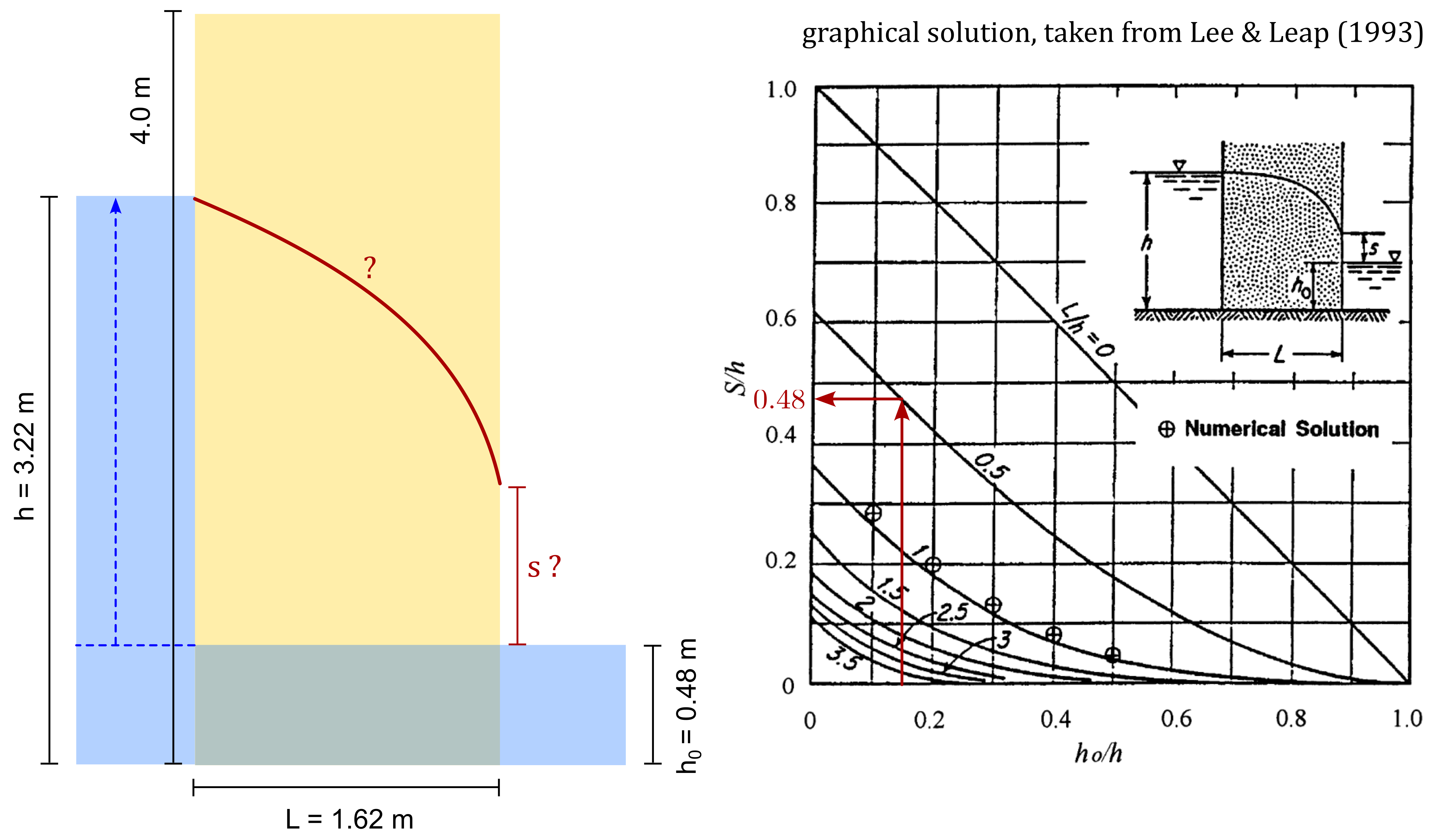Figure 1. Problem statement unconfined groundwater flow, Right: Graphical solution for the estimation of the seepage face height $s$ according to Lee and Leap (1997)².

The displacements are constrained at all nodes (only the flow of water is investigated in this example). The initial pore water pressure is assumed to be linearly distributed with the water table located at 0.48 m above the bottom boundary. Above 0.48 m the soil is initially partially saturated. During the analysis, the water table on left side of the dam is elevated up to a height of 3.22 m above the bottom boundary of the model.

The distribution of the phreatic surface in the dam and the height of the seepage face (size of the saturated area above the water table on the right-hand side of the dam) are the sought-after variables of this simulation.

The finite element model including information about later used set names as well as the initial distribution of pore water pressure $p^w$ and degree of saturation $S^w$.

Figure 2. Finite element model and initial conditions.

The soil was discretized using stabilized linear elements for the simulation of partially saturated soils. These elements use equal order interpolation for the displacements (u) and pore water pressures (p). The corresponding element types are u3p3-stab and u4p4-stab-red for the triangular and rectangular elements, respectively. The keyword stab refers to the use of stabilisation techniques to allow for the use of equal order interpolation without suffering from oscillations in pore water pressure $p^w$ due to the violation of the LBB (inf-sup) condition. The keyword red refers to the use of reduced integration, i.e. a single integration point located in the center of the element is used for the numerical integration of the u4p4-stab-red element.

Simplified element formulation

With above element choice, changes in pore air pressure are judged as negligible, a reduced set of governing equations is used - namely the up-formulation. These elements consider negative pore water pressures as suction $s=-p^w$ (instead of calculating it from the pore water pressure and the pore air pressure $p^a$ as $s=p^a-p^w$).

Material definition

For the solid a linear elastic constitutive model is chosen. As no soil deformation is considered in this simulation this choice is completely arbitrary. The Young's modulus is 50 MPa and the Poisson's ratio $0.3$. No information about the bulk modulus of the pore water $K^w$ is provided, thus the bulk modulus is assumed to correspond to the one of pure water $K^w = 2.2\cdot 10^6$ kPa. The density of the grains, water and air are assumed to be $\rho^s=2.65$ t/m³, $\rho^w=1.0$ t/m³ and $\rho^a=0.0015$ t/m³.

*Material, name = elastic, phases = 3
*Mechanical = linear_elasticity
50d3, 0.3
*Density
2.65, 1.0, 0.0015
*Bulk modulus
2.2d6, 100.

Both the soil-water-retention curve and the dependence of the relative permeability on the effective degree of saturation are modelled using the well known van Genuchten model. The hydraulic conductivity $K$ and the parameters of the van Genuchten model are chosen to: $K= 1.7604 \cdot 10^{-6}$ m/s, $n^{vG} = 1.377$ and $\alpha^{vG}=0.383$. The residual degree of saturation is $S^{res}=0.063$.

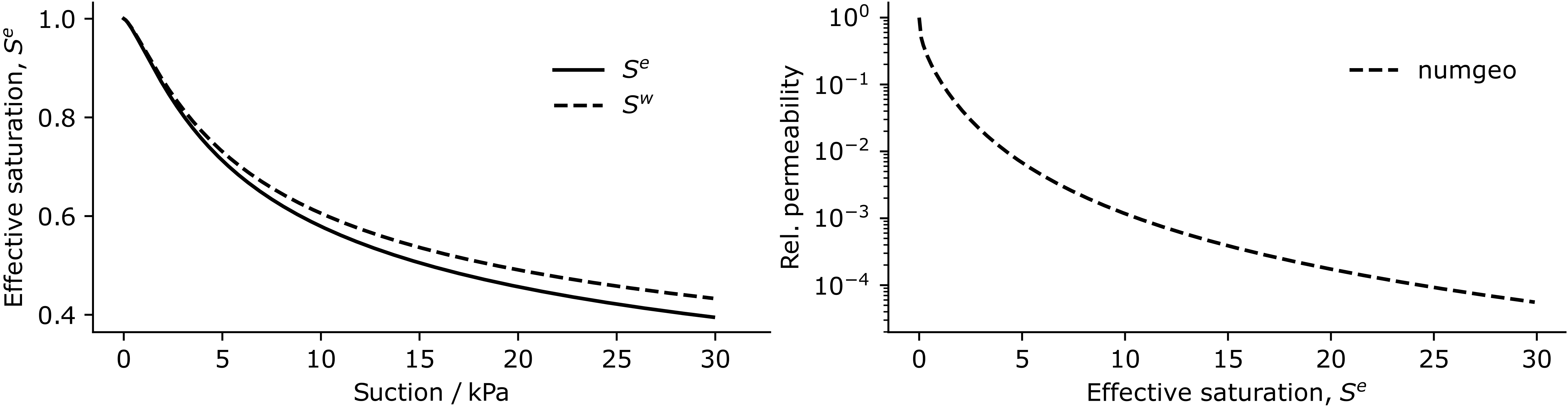Soil-water-retention curve and relative permeability used for the simulation

The corresponding code for the specification of the hydraulic models and the permeability is given below.

*Dynamic viscosity
1d-6, 1d-8

*Permeability = isotropic
1.157407d-12

*Hydraulic = van Genuchten, Swr=0.063
0.383, 1.377
*Jacobian = Smoothed

*Relative permeability = van Genuchten
1d-6, 1d-6, 1.377

Permeability vs. hydraulic conductivity

Note that numgeo requires the prescription of the permeability $K^s$ of the solid and the dynamic viscosity of the pore fluids $\mu^f$ instead of the hydraulic conductivity $K^f$, which are related as follows: $$ K^f = \dfrac{K^s \gamma^f}{\mu^f} $$

Therein, $\gamma^f$ and $\mu^f$ are the specific weight and the dynamic viscosity of the fluid $f$, respectively.

The dynamic viscosity of pore water is $\mu^w=10^{-6}$ m$\cdot$s and of the pore air $\mu^a=10^{-8}$ m$\cdot$s. Assuming a specific weight of 10 kN/m$^3$ for the pore water, the permeability of the soil is calculated to $1.157407 \cdot 10^{-12}$ m$^2$.

Since the calculation of changes in effective stress are not of interest in this example, we neglect the contribution of the capillary pressure $p^c=-p^w$ to the effective stress by choosing the crude-switch option for the Bishop effective stress:

*Bishop effective stress = Crude-Switch

Initial conditions

For the initial pore water pressure the water level is assumed to be located at a height of 0.48 m above the bottom of the model. This results in a linear distribution of pore water pressure taking values of $p^w_0=4.8$ kPa at the bottom, $p^w_0=0$ kPa at 0.48 m and $p^w_0=-35.2$ kPa at the top of the dam.

*Initial conditions, type=pore water pressure, default
Soil.all, 0.0d0, 4.8d0, 4.d0, -35.2d0

The initial void ratio is $e_0 = 0.5$.

*Initial conditions, type=void ratio, default
Soil.all, 0.5

Although it is not theoretically necessary for this simulation, we also define the initial stress state. The reason for this is that numgeo expects an initial stress to be specified for elements that discretise displacement as a degree of freedom. As this is of no further importance here, we initialise it to zero.

*Initial conditions, type=stress, geostatic
Soil.all, 0.0, 0.0, 4.0, 0.0, 0.0, 0.0

Geostatic step

During the Geostatic step, the self weight of the soil (grains and pore water) is applied without generating any deformation. A gravitational body force of $g=10$ m/s² acting in vertical (y) direction is considered. As stated previously, no deformation of the soil skeleton is expected. We therefore constrain the displacements of all nodes in $x$ and $y$ direction. In addition, we use boundary conditions to prescribe the pore water pressure. As in the initial conditions, the pore water pressure is assumed to vary linearly with depth for which the hydrostatic option is used.

*Step, name=Geostatic, inc=1, maxiter=100
*Geostatic

*Body force, instant
Soil.all, grav, 10.0, 0., -1, 0.

*Boundary
Soil.all, u1, 0.
Soil.all, u2, 0.

*Boundary, type=hydrostatic
Soil.all, pw, 10.0, 0.48

Next we define which quantities we want to display as a result of the simulation. For this example, we are interested in the degree of saturation sat (calculated and stored at the element level) and the pore water pressure pw (calculated and stored at the nodes). The step definition is closed by *End Step.

*Output, field, vtk, ascii
*Element, elset = Soil.all
sat
*Node, nset = Soil.all
pw

*End Step

Transient step

During the transient step we simulate the water supply at the left side of the dam. This is done by prescribing the pore water pressure at the corresponding nodes using a user defined subroutine. The total step time is chosen 172,800 seconds, corresponding to 2 days. Due to the strong non-linearities resulting from the saturation-suction relation and the relative permeability function, we limit the maximum allowed time increment size to 1000 seconds.

*Step, name=Saturation, inc=1000000, maxiter=50

*Transient
100, 172800, 1, 1000

*Body force, instant
Soil.all, grav, 10.0, 0., -1, 0.

*Boundary
Soil.all, u1, 0.
Soil.all, u2, 0.

During the transient step, the water level on the left-hand-side of the model Soil.left_sat is increased from initially 0.48 m to 3.22 m over a time period of 2.4 hours (8,640 seconds). Since the prescribed pore water pressure not only varies with time but also in space $\tilde{p}^w(y,t)$ we use a user-defined boundary condition *UBoundary. On the right-hand-side (Soil.right_sat) the water level stays at 0.48 m which is enforced using a boundary condition.

*UBoundary
Soil.left_sat, pw, 1.

*Boundary, type=hydrostatic
Soil.right_sat, pw, 10.0, 0.48

The increase in pore water pressure can be described using the following relation

\[ \tilde{p}^w(y,t) = \begin{cases} p^w_0 + (p^w_{end}-p^w_0)t & \text{for}~ t < t_{end} \\ p^w_{end} & \text{else} \end{cases} \]

where $p^w_0$ is the initial pore water pressure at position $y$, $t$ is the current simulation time, $t_{end}=2.4$ hours and $p^w_{end}(y) = (3.22\text{m} - y)\gamma^w$. $y$ is the y-coordinate of the current node under consideration and $\gamma^w=10$ kN/m³ is the specific weight of water. The corresponding Fortran code is given in below Section. For an introduction to the use of user-defined routines it is referred to User defined extensions

A special boundary condition is needed if the phreatic surface reaches an open, freely draining surface. In the present simulation this is the case on the right-hand-side of the model since the seepage height $s$ varies with time until it eventually reaches its final value. In such a case the pore fluid can drain freely down the face of the dam, so $p^w=0$ at all points on this surface below its intersection with the phreatic surface. Above this point negative pore water pressures occur, with their particular value depending on the solution. This drainage-only flow condition consists of prescribing the flow velocity on the freely draining surface in a way that approximately satisfies the requirement of $p^w=0$ on the completely saturated portion of this surface:

\[ q^w = \begin{cases} \tilde{k}_s \left(p^w - p^w_{target} \right) & \text{if}~~ p^w > p^w_{target} \\ 0 & \text{else}\end{cases} \]

where $p^w_{target}$ is the target pore water pressure at the considered surface and $\tilde{k}_s$ is the proportionality coefficient. In the present case $p^w_{target}=0$ kPa and $\tilde{k}_s$ can be estimated based on the characteristic element size $c=0.1$ m, the saturated hydraulic conductivity $K$ and the specific unit weight of pore water $\gamma^w=10$ kN/m³ as $\tilde{k}_s = 10^5 K/\gamma^w c \approx 0.002$ m³/Ns.

In numgeo this can be realized using the *DSLoad option:

*DSload, instant
surf_right, drainage-w, 0.002

Finally, we enable the convergence controls of the pore water pressure and disable the "global" convergence controls. The step is closed with *End Step and the input file with *End Input

*controls, global, deactivate
*controls, pw, activate
*End Step
*End Input

Results

The following figure presents the the simulation results obtained with numgeo for three different meshes by means of the distribution of pore water pressure in steady state conditions. Following the phreatic surface (line/surface at which $p^w=0$ kPa holds) the seepage face $s$ can be identified. The calculated seepage face by means of FEM fit reasonably well to the reference analytical solution (Muskat).

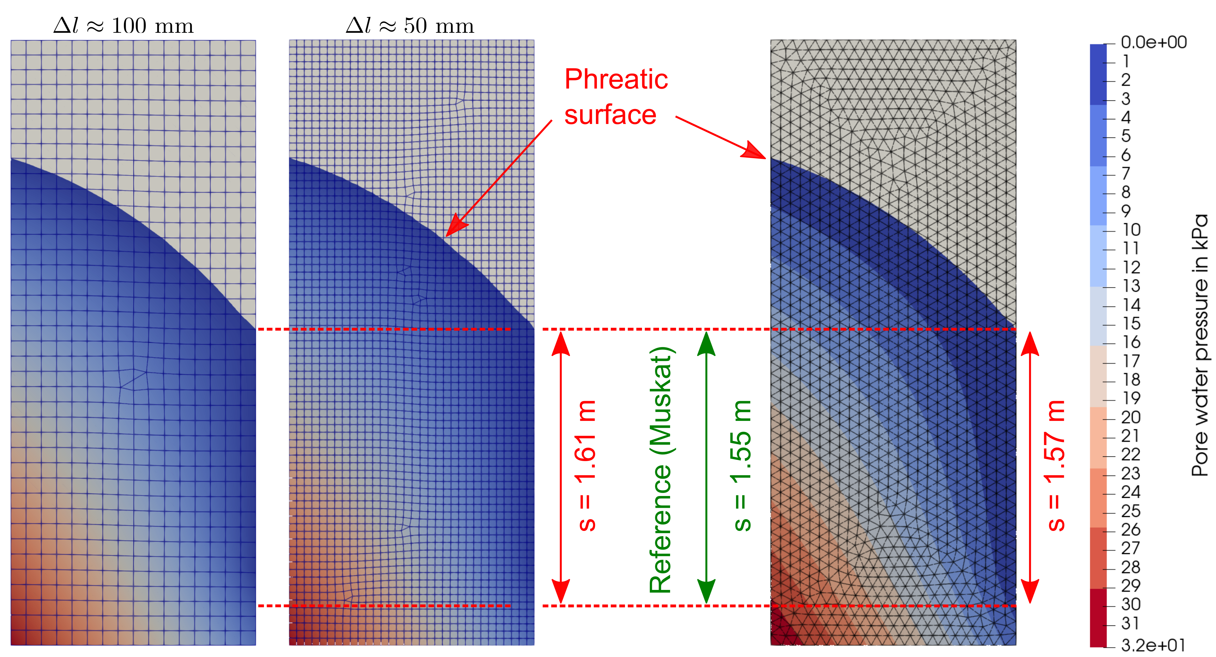Distribution of pore water pressure obtained by Plaxis (left) and numgeo (right) as well as height of the seepage face $s$ (m).

User-defined boundary condition

Windows

subroutine user_boundary_conditions(dof,inode,istep,time,coords,bc_value) 
  implicit none
  !DEC$ ATTRIBUTES DLLEXPORT, STDCALL, REFERENCE :: user_boundary_conditions
  character            , intent(in)    :: dof          !! degree of freedomn for which the boundary condition is defined
  integer              , intent(in)    :: inode        !! node label
  integer              , intent(in)    :: istep        !! (current) step number
  real(8)              , intent(in)    :: time         !! step time
  real(8), dimension(3), intent(in)    :: coords       !! coordinates of the integration point
  real(8), dimension(3), intent(inout) :: bc_value     !! initial stress

    real(8) :: gammaW, pw_0, final_pw, rising_time, m

    gammaW = 10.0d0
    rising_time = 0.1d0 * 24.0d0 * 60.0d0 * 60.0d0
    if(istep == 2) then
      pw_0 = - (coords(2)-0.48)*gammaW
    final_pw = (3.22d0-coords(2)) * gammaW
    if (time < rising_time) then
      m = (final_pw-pw_0)/rising_time
      bc_value(1) = pw_0 + m*time
    else
      bc_value(1) = final_pw
      end if
    endif

end subroutine user_boundary_conditions

Linux

subroutine user_boundary_conditions(dof,inode,istep,time,coords,bc_value) bind(c,name='user_boundary_conditions')
  use, intrinsic :: iso_c_binding
  implicit none
  character(c_char)           , intent(in)    :: dof          !! degree of freedomn for which the boundary condition is defined
  integer(c_int)              , intent(in)    :: inode        !! node label
  integer(c_int)              , intent(in)    :: istep        !! (current) step number
  real(c_double)              , intent(in)    :: time         !! step time
  real(c_double), dimension(3), intent(in)    :: coords       !! coordinates of the integration point
  real(c_double), dimension(3), intent(inout) :: bc_value     !! initial stress

    real(8) :: gammaW, pw_0, final_pw, rising_time, m

    gammaW = 10.0d0
    rising_time = 0.1d0 * 24.0d0 * 60.0d0 * 60.0d0
    if(istep == 2) then
      pw_0 = - (coords(2)-0.48)*gammaW
    final_pw = (3.22d0-coords(2)) * gammaW
    if (time < rising_time) then
      m = (final_pw-pw_0)/rising_time
      bc_value(1) = pw_0 + m*time
    else
      bc_value(1) = final_pw
      end if
    endif

end subroutine user_boundary_conditions

P. Y. Polubarinova-Kochina, Theory of ground water movement. Princeton university press, 1962. ↩↩
K.-K. Lee and D. I. Leap, ‘Simulation of a free-surface and seepage face using boundary-fitted coordinate system method’, Journal of Hydrology, vol. 196, no. 1–4, pp. 297–309, Sep. 1997, doi: 10.1016/S0022-1694(96)03246-5. ↩↩