Vertical cut slope (Byun 2019)
Quick read on strength-reduction analysis
The strength reduction method is a separate calculation type that can be selected using the keyword *Reduction in the step definition. During a strength reduction analysis, the shear strength parameters of the soil are incrementally reduced in accordance with a strength reduction factor (SRF) until failure is obtained. The SRF is applied to the tangent of the friction angle and the cohesion to ensure equal proportion of shear resistances by frictional and cohesive terms throughout the strength reduction. Assuming that the factor of safety (FoS) is identical to the SRF, the reduced shear strength parameters \(\varphi_\text{red}\) and \(c_\text{red}\) can be determined based on the actual shear strength parameters and the FoS as follows:
\(\tan \varphi_\text{red} = \tan \varphi\,/\,\text{FoS} \qquad \text{and} \qquad c_\text{red} = c\,/\,\text{FoS}\)
To control the incremental reduction of the shear strength parameters, the line following the keyword *Reduction requires the definition of four scalars: an initial value of the factor of safety (FoS\(_0\)) and an initial step-size (\(\Delta\)FoS\(_0\)), a maximum step-size (\(\Delta\)FoS\(_{\max}\)) and a minimum step-size (\(\Delta\)FoS\(_{\min}\)) need to be prescribed in the calculation type definition. During a strength reduction analysis, FoS is incrementally increased, which results in an incremental reduction of the shear strength parameters.
The strength reduction method can be used in combination with the Mohr-Coulomb and Matsuoka-Nakai model, so far. To specify that the shear strength parameters of a specific material parameter set should be reduced during a strength reduction analysis, the keyword *Reducible Strength needs to be specified in the material definition.
Detection of failure is conducted based on non-convergence. Moreover, post-processing can be used additionally to inspect the maximum displacements vs. FoS. Plotting the former in logarithmic scale, slope failure can also be defined as the FoS associated to a decisive kink in the curve trend.
The second tutorial on strength reduction features a boundary value problem presented by Byun (2019)1 who compared the performance of the geotechnical finite element software products Plaxis, ZSoil and GEO5 and others (no name provided). Amongst other, the stability of a vertical cut slope was analysed using the strength reduction method. The geometry and finite element mesh are shown in Figure 1.
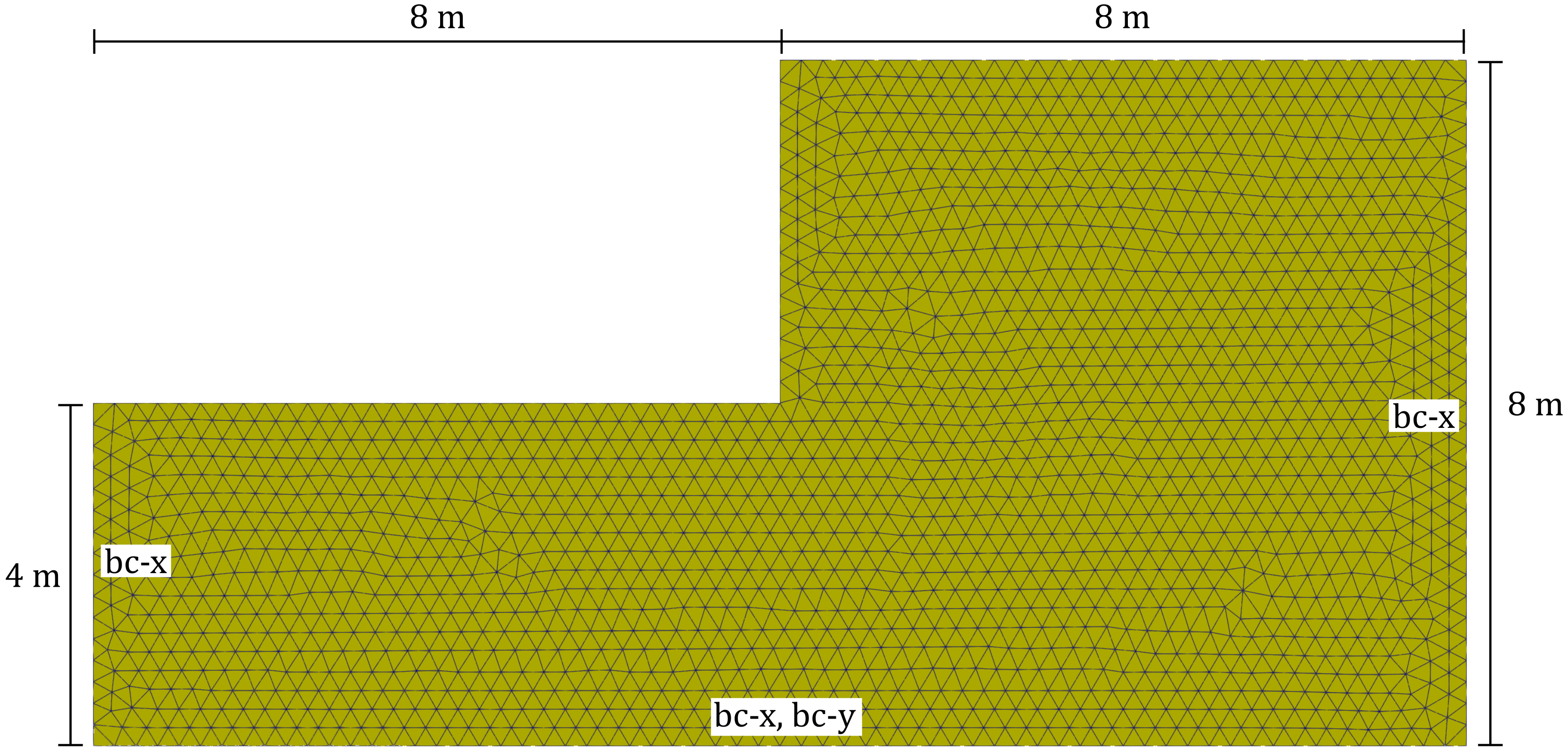
Figure 1. Problem setting and representative finite element mesh of the homogeneous slope used in this tutorial.
The linear elastic, perfectly plastic Mohr-Coulomb (M-C) model was used in the analysis. The material properties are as follows:
Table 1. Material parameters for the strength-reduction analyses
| \(E\) (kPa) | \(\nu\) | c (kPa) | \(\varphi\) (°) | \(\rho\) (t/m³) |
|---|---|---|---|---|
| 30000 | 0.3 | 16 | 30 | 1.6 |
where \(E\) denotes the Young's modulus, \(\nu\) the Poisson's ratio, \(c\) the effective cohesion and \(\varphi\) the effective friction angle, respectively. \(\rho\) is the density of the soil. The dilatation angle is assumed as \(\psi=0\)°. No tension cut-off is used. For the back-calculation we will use the Mohr-Coulomb-3 model.
Input files
The input files for the tutorial can be downloaded here.
Finite element mesh
The finite element model was created using the GiD pre-processing software, the corresponding GiD (GUI) files from here. For the discretisation of the domain, two-dimensional u-solid finite elements are used, discretising the displacement (u) of the solid. The mesh is composed of 6-noded triangular elements with quadratic interpolation order (termed u6-solid).
.
.
*Element, Type = U6-solid
.
.
In the mesh file, node sets (NSet) and element sets (ElSet) have been defined to address groups of nodes and elements to be used in the step files (e.g. for the definition of boundary conditions). The following node sets have been defined in the mesh file and used in the step files: bc-x, bc-y, all. Only one element set has been defined: all. For bc-x and bc-y see also Figure 1
To keep the input file as short as possible, we store the finite element mesh in a separate file byun-2019-mesh.inp and import it at the beginning of the actual input file byun-2019.inp containing the material and calculation specifications:
*Include = byun-2019-mesh
*Include = byun-2019-mesh
Material definition
The material behavior of the soil is described by the Mohr-Coulomb model with material parameters selected as provided in Table 1. We recommend the use of the Mohr-Coulomb-3 implementation. The material model requires the definition of a tension cut-off. Since in this problem statement no tension cut-off is used, we simply prescribe the apex of the Mohr Coulomb criterion as tension cut-off:
\(p_t = \dfrac{c}{\tan \varphi} = 27.7\) kPa
To consider that shear strength parameters of a specific material parameter set should be reduced in a strength reduction analysis, the keyword *Reducible Strength needs to be specified in the material definition.
*Material, name=Material 1, phases=1
*Mechanical = Mohr-Coulomb-3
30000, 0.3, 16, 30, 0, 27.7
*Density
1.6
*Reducible Strength
Initial conditions
The initial state assumes a horizontal ground surface at a height of 8 m. A lithostatic initial (effective) stress and \(K_0=0.5\) are assumed:
*initial conditions, type=stress, geostatic
all, 0, -128, 8, 0, 0.5, 0.5
Amplitudes
Amplitudes need to be defined to allow for changes of loads or boundary conditions during a step. For this example, only an unloading ramp is needed to incrementally decrease the reaction forces at the nodes in Step 2.
*Amplitude, name = UnloadingRamp, type = Ramp
0.0, 1.0, 1.0, 0.0
Steps
The simulation consists of a total of three steps which are explained in the following sections.
Step 1
The first step is conducted in terms of a *Geostatic step. In this step, the initial stress distribution defined in the initial conditions is considered and deformations of all nodes are restricted in x- and y-direction, allowing for no deformations in the entire model. The reaction forces associated to the restricted degrees of freedom (DOF) at all nodes are saved. VTK output files are generated to allow for post-processing with Paraview.
*Step, name=Step 1, inc=1e4, maxiter=32, miniter=1
*Geostatic
*Boundary
all, u1, 0
all, u2, 0
*Save Reaction force
all, 1
*Save Reaction force
all, 2
*Body force, instant
all, Grav, 10, 0.0,-1.0,0.0
*output, field, VTK, ASCII
*frequency=1
*node output, nset = all
u, S, e,  FoS
*End Step
Step 2
The second step is performed as a *Static step. In this step, the reaction forces are gradually reduced to zero, allowing for the system to deform and find an equilibrium stress state by developing shear stresses. The boundary conditions are modified such that lateral deformations are restricted at the left and right boundaries and lateral and vertical deformations are restricted at the bottom boundary of the model.
*Step, name=Step 2, inc=1e4, maxiter=32, miniter=1
*Static
0.01, 1, 0.001, 0.1
*Boundary
bc-x, u1, 0
*Boundary
bc-y, u2, 0
*Reaction force, amplitude=unloading
all, 1
*Reaction force, amplitude=unloading
all, 2
*Body force, instant
all, Grav, 10, 0.0,-1.0,0.0
*output, field, VTK, ASCII
*frequency=1
*node output, nset = all
u, S, e,  FoS
*End Step
Step 2
In the second step we perform the strength reduction simulation. With the keyword *Reduction, numgeo uses an automatic procedure to determine the Factor of Safety (FoS) for the current system by incrementally decreasing (and increasing) the shear strength parameters.
*Step, name=Step 3, inc=1e4, maxiter=16, miniter=1
*Reduction
1.0, 0.05, 0.05, 0.0001
*Boundary
bc-x, u1, 0
*Boundary
bc-y, u2, 0
*Reset
Displacement, Strain
*Body force, instant
all, Grav, 10, 0.0,-1.0,0.0
*output, field, VTK, ASCII
*frequency=1
*node output, nset = all
u, S, e,  FoS
*End Step
At the end, we close the input file with the following command:
*End Input
Results
The displacement contour plot is depicted in Figure 2. The simulation results show a clear failure mechanism resembling a linear failure plane.
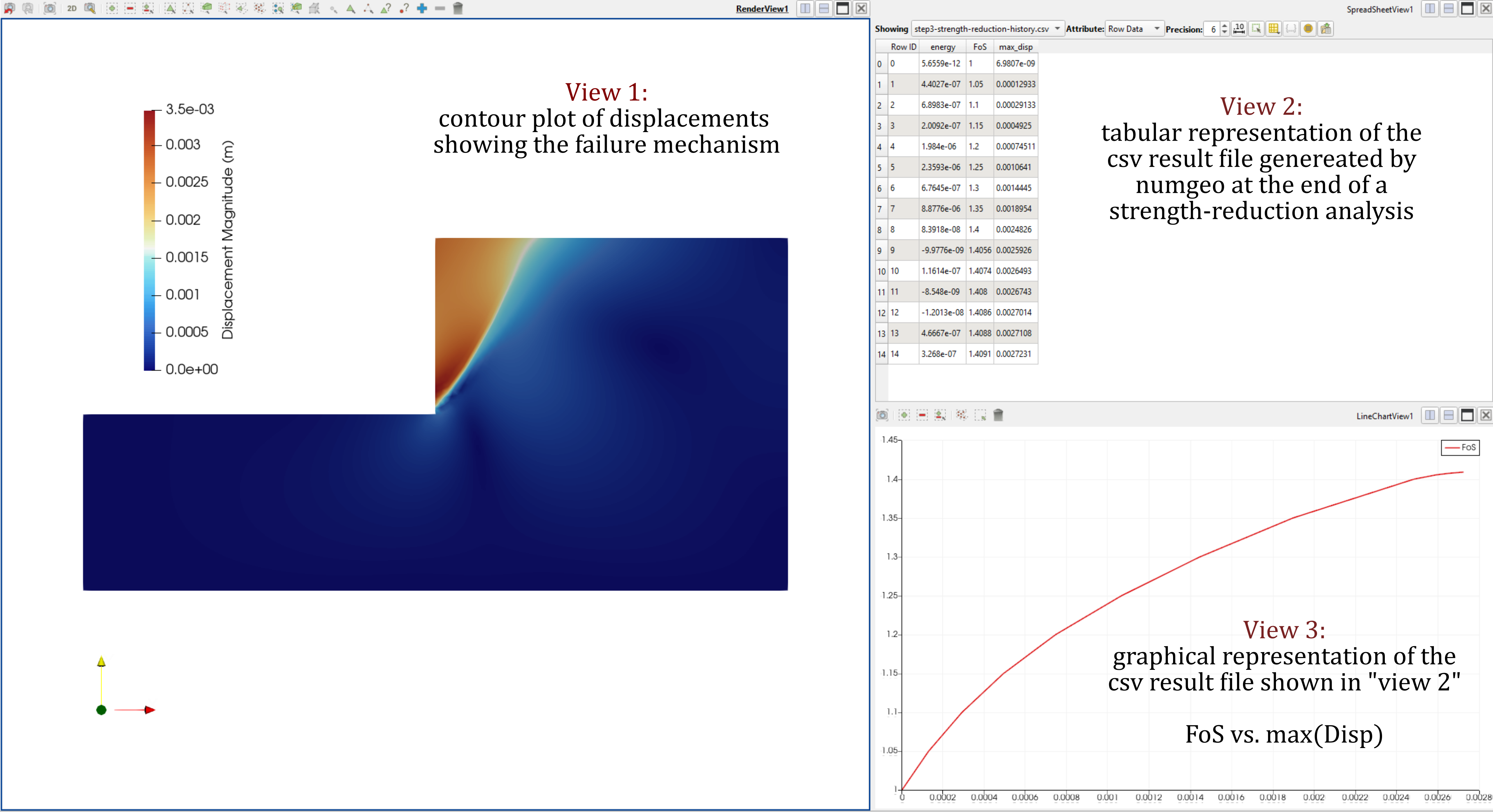
Figure 2. Simualtion results in Paraview: Displacement contour plot (left), FoS vs. max. displacement magnitude as tabular data (top right) or as xy-plot (bottom right).
The FoS, max. displacement magnitude and internal energy data are saved as an output automatically by numgeo at the end of a strength-reduction analysis and saved in a csv file, here named step3-strength-reduction-history.csv. Such a file can also be imported into Paraview and displayed as tabular data (View 2) or as plotted as xy-data, here as FoS vs. the maximum displacement magnitude (View 3).
The resulting Factor of Safety (FoS) obtained with numgeo is compared to the results of the five different software packages (and analysis methods) in Figure 3. It can be seen that the results obtained with numgeo are within the range of results obtained with other software and are close to the once obtained with Plaxis.
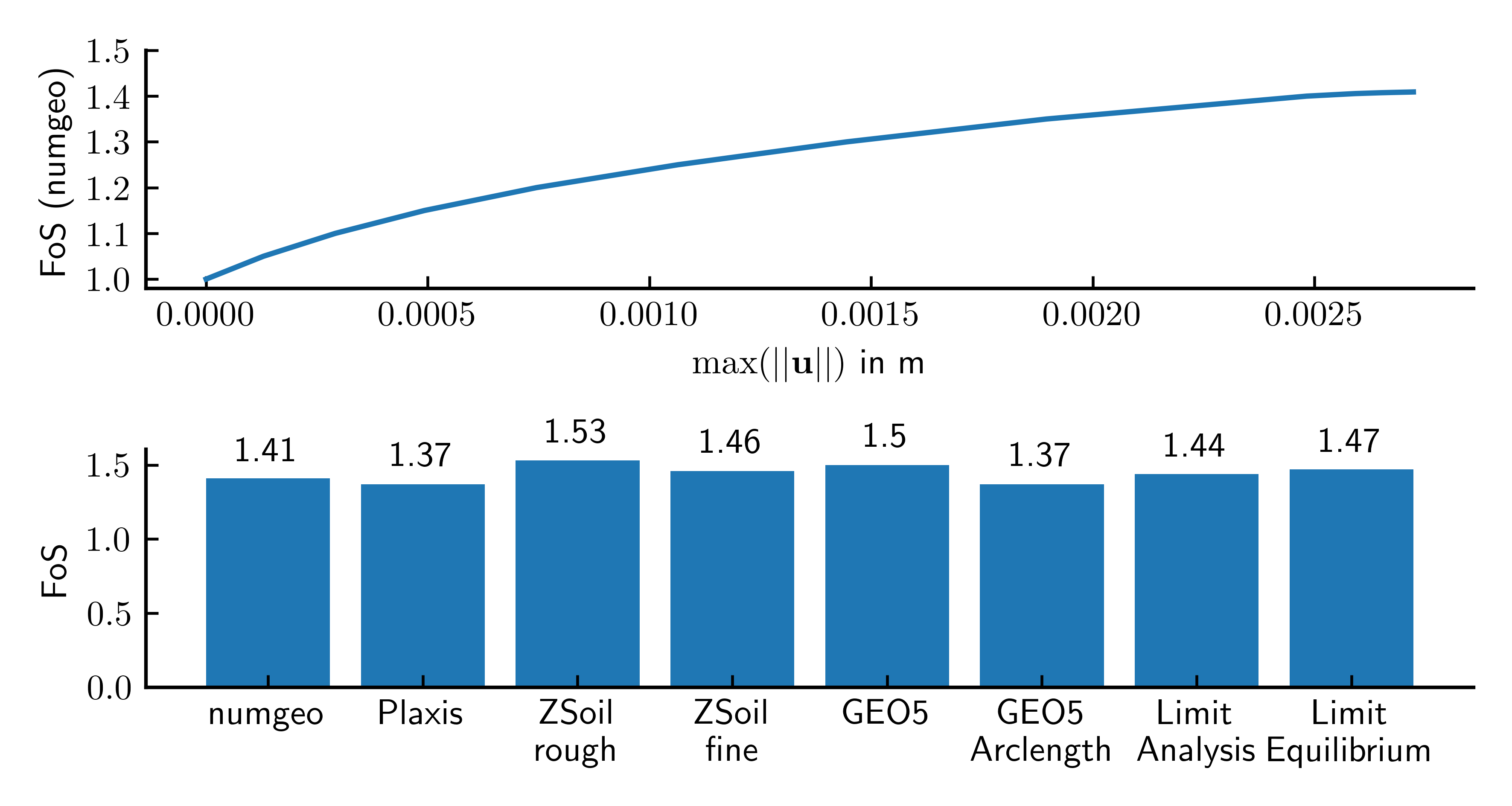
Figure 3. Max. displacement magnitude versus Factor of Safety (FoS) for case 1, calculated with numgeo (top) and comparison to other software (bottom).
The python script used to produce this plot is given below.
#%%
import numpy as np
import matplotlib.pyplot as plt

fontsize = 10
plt.rcParams['xtick.direction'] = 'in'
plt.rcParams['ytick.direction'] = 'in'
plt.rcParams['text.usetex'] = True
plt.rcParams['font.size'] = fontsize
plt.rcParams['axes.spines.right'] = False
plt.rcParams['axes.spines.top'] = False
plt.rcParams['axes.linewidth'] = 1.0

# Convert centimeters to inches for figure sizing
def cm2inch(*tupl):
    inch = 2.54
    if isinstance(tupl[0], tuple):
        return tuple(i/inch for i in tupl[0])
    else:
        return tuple(i/inch for i in tupl)

data = np.genfromtxt('./step3-strength-reduction-history.csv', delimiter=',')

fig, ax = plt.subplots(2,1, figsize=cm2inch(15,8), sharex=False)

ax[0].plot(data[:,1],data[:,0])
ax[0].set_xlabel('$\max(||\mathbf{u}||)$ in m')
ax[0].set_ylabel('FoS (numgeo)')
ax[0].set_yticks([1., 1.1, 1.2, 1.3, 1.4, 1.5])

fos = [np.round(data[-1,0],2), 1.37, 1.53, 1.46, 1.5, 1.37, 1.44, 1.47]
labels = ['numgeo','Plaxis', 'ZSoil \n rough', 'ZSoil \n fine', 'GEO5', 'GEO5 \n Arclength', 'Limit \n Analysis', 'Limit \n Equilibrium']

rects = ax[1].bar(labels, fos)
ax[1].bar_label(rects, padding=3)
ax[1].set_ylabel('FoS')
ax[1].set_yticks([0.0, 0.5, 1.0, 1.5])

plt.tight_layout()

plt.savefig('./byun-2019-results-plot.png', dpi=600)
-
G. W. Byun. Comparison between Geotechnical Softwares. In ZSoil Day 2019. 2019-09-25. URL: https://www.zsoil.com/zsoil_day/2019/GW_Byun_Comparision_Geotech_Softwares_2019.pdf. ↩