Saturated elastic soil

The input files can be downloaded here.

To study the effect of the pore water pressure change and consolidation, a simulation incorporating so called coupled elements is conducted. Coupled elements do not only discretise the displacement of the solid phase but also the pore water pressure (u-p elements), the displacement of the water (u-U elements) or both the pore water pressure and the displacement of the water (u-p-U elements). For the present simulation, the u-p elements will be used.

The ground water level will be set to the ground surface and drainage alongside the top surface will be assumed. The load of the foundation is again applied within 1 s (physical time now since a transient process is studied). After the application of the load, the consolidation process (the dissipation of the excess pore water pressure built under the foundation due to the loading) is studied in a third step in which a time span of 100,000 s is considered.

Definitions in the input file

Use the input files from the dry calculation, search in "Mesh_Soil" from the top for the keyword Element. Change the element type to

*Element, Type = u8p4-sat

u8p4-sat elements (the element has 8 nodes with solid displacement degree of freedoms (dofs), 4 pore water pressure dofs and assumes a fully saturated state (-sat)) are used.

The material definition of the soil has to be changed in order to define a two-phase material (solid grains plus water) now:

**
** Material
**

*Material, name = soil, phases = 2
*Mechanical = Linear_Elasticity
10000, 0.3
*Density
2.65,1.0

*Bulk modulus
2.2d6

*Permeability = isotropic
1.0d-12

*dynamic viscosity
1d-6
**

Here, two densities have to be given which are the density of the solid grains and the density of water. In addition, the bulk modulus of the pore water and the permeability have to be defined. In numgeo, the permeability equals the dynamic viscosity (set to \(10^{-6}\) kPas) multiplied with the hydraulic conductivity \(k^w\) and divided by the unit weight of water (\(\gamma_w = 10~\)kN/m\(^3\)). A hydraulic conductivity of \(k^w\) = 1 \(\cdot\) \(10^{-5}\) m/s is defined here. The resulting permeability of \(10^{-12}\) is define using *Permeability = isotropic.

Using two-phase elements, the definition of an initial void ratio is required, which is used to calculate the effective weight:

**
** Initial conditions
**

*initial conditions, type=void ratio, default
Soil.all, 1.0d0

In addition, the initial pore water pressure has to be set:

*initial conditions, type=pore water pressure, default
Soil.all, 0.0d0, 100.0d0, 10.0d0, 0.0d0

Since effective stresses are used now, the initial stress condition of the soil has to be changed:

*initial conditions, type=stress, geostatic
Soil.all, 10, 0, 0, -82.5, 0.5, 0.5

Therein the element set \(all\_soil\) is assigned an initial effective stress state with \(\sigma_{22}(y=0.0\) m\()=-82.5\) kPa (since \(\gamma' = (1-n)\cdot(\gamma_s -\gamma_w) = \big(1-\dfrac{e}{1+e}\big)\cdot\big(\gamma_s -\gamma_w\big)=8.25\) kN/m\(^3\)) and \(\sigma_{22}(y=10.0\) m\()=0.0\) kPa.

In the first step, only little changes have to be made compared to the dry case:

**
** Load step 1
**

*Step, name=step1, inc = 1
*Geostatic

*Body force, instant
Soil.all, GRAV, 9.99, 0, -1, 0
*Body force, instant
Foundation.all, GRAV, 9.99, 0, -1, 0

*Boundary
Foundation.all,u1, 0.0d0
Foundation.all,u2,0.0d0
Soil.left,u1,0.0d0
Soil.right,u1,0.0d0
Soil.bottom,u2,0.0d0

*Boundary,type=hydrostatic
Soil.all,pw, 10, 10

*output, field, vtk, ASCII
*node output, nset = Soil.all
U, pw
*element output, elset = Soil.all
S, Contact

*End Step

The boundary condition for the pore water pressure is added. A hydrostatic distribution is defined for all soil nodes. The distribution defined here coincides with the defined initial conditions. The first value is the unit weight of water \(\gamma_w\) and the second "10" is the height of the ground water level. This defines a linear distribution of pore water pressure. For the output the pore water pressure is added using Pw.

The second step is defined as follows:

**
** Load step 2
**

*Step, name=step2, inc = 10000
*transient
0.01,1.0,0.0001,0.01

*Body force, instant
Soil.all, GRAV, 9.99, 0, -1, 0
*Body force, instant
Foundation.all, GRAV, 9.99, 0, -1, 0

*Boundary
Foundation.left, u1, 0.0d0
Soil.left,u1,0.0d0
Soil.right,u1,0.0d0
Soil.bottom,u2,0.0d0
Soil.top,pw,0.0d0

*DSload, amplitude = LoadingRamp
surf_foundation_top, p, -100.0d0

*Controls, global, deactivate
*Controls, u, activate

*Output, field, vtk, ASCII
*Node output, nset = Soil.all
U, pw
*Element output, elset = Soil.all
S, Contact

*Output,print
*frequency = 1
*Node output, nset = Foundation.top_left_node
U 

*End Step

In comparison to the dry simulation, the type of analysis was changed to a transient calculation, including pore water pressure change and water flow (consolidation). Note that physical time is now used for this step. Therefore, the step is 1 s long. The boundary conditions for the pore water pressure of the soil is now redefined for the top node set only. This means that this edge is now permeable and open for water flow. The pore water pressure is added to the nodal output. The rest of the step remains the same as in the dry case. The load on the foundation is reduced to 100 kPa compared to the example with dry soil.

To study the consolidation process after the load of the foundation is applied, a third step is created:

**
** Load step 3
**

*Step, name=step3, inc = 100000
*transient
0.1,1d5,0.0001,2000

*Body force, instant
Soil.all, GRAV, 9.99, 0, -1, 0
*Body force, instant
Foundation.all, GRAV, 9.99, 0, -1, 0

*Boundary
Foundation.left, u1, 0.0d0
Soil.left,u1,0.0d0
Soil.right,u1,0.0d0
Soil.bottom,u2,0.0d0
Soil.top,pw,0.0d0

*DSload, instant
surf_foundation_top, p, -100.0d0

*Controls, global, deactivate
*Controls, u, activate

*Output, field, vtk, ASCII
*Node output, nset = Soil.all
U, pw
*Element output, elset = Soil.all
S, Contact

*Output,print
*frequency = 1
*Node output, nset = Foundation.top_left_node
U

*End Step

The total time of this step is 100,000 s and the maximum time increment is 2000 s. The load of the foundation is now applied instantly, as the load was already brought into equilibrium with the model in the second step.

Results of the simulation

The results of the field of pore water pressure at the end of step 2 are shown in Figure 1. Since the entire top of the soil is permeable, zero pore water pressure is encountered directly under the foundation.

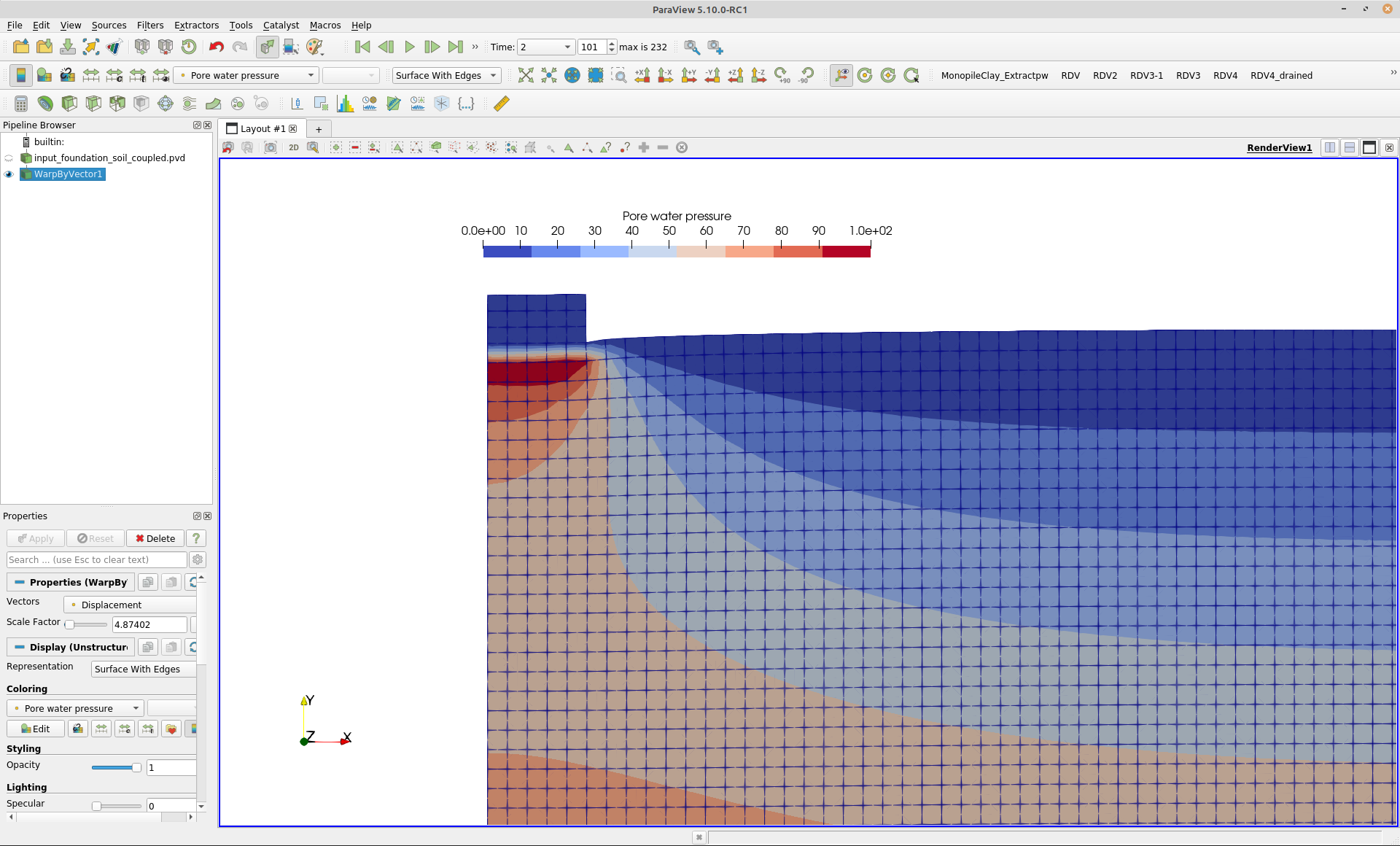Figure 1. Pore water pressure after application of the foundation load

Figure 2 shows the vertical displacement of the foundation.

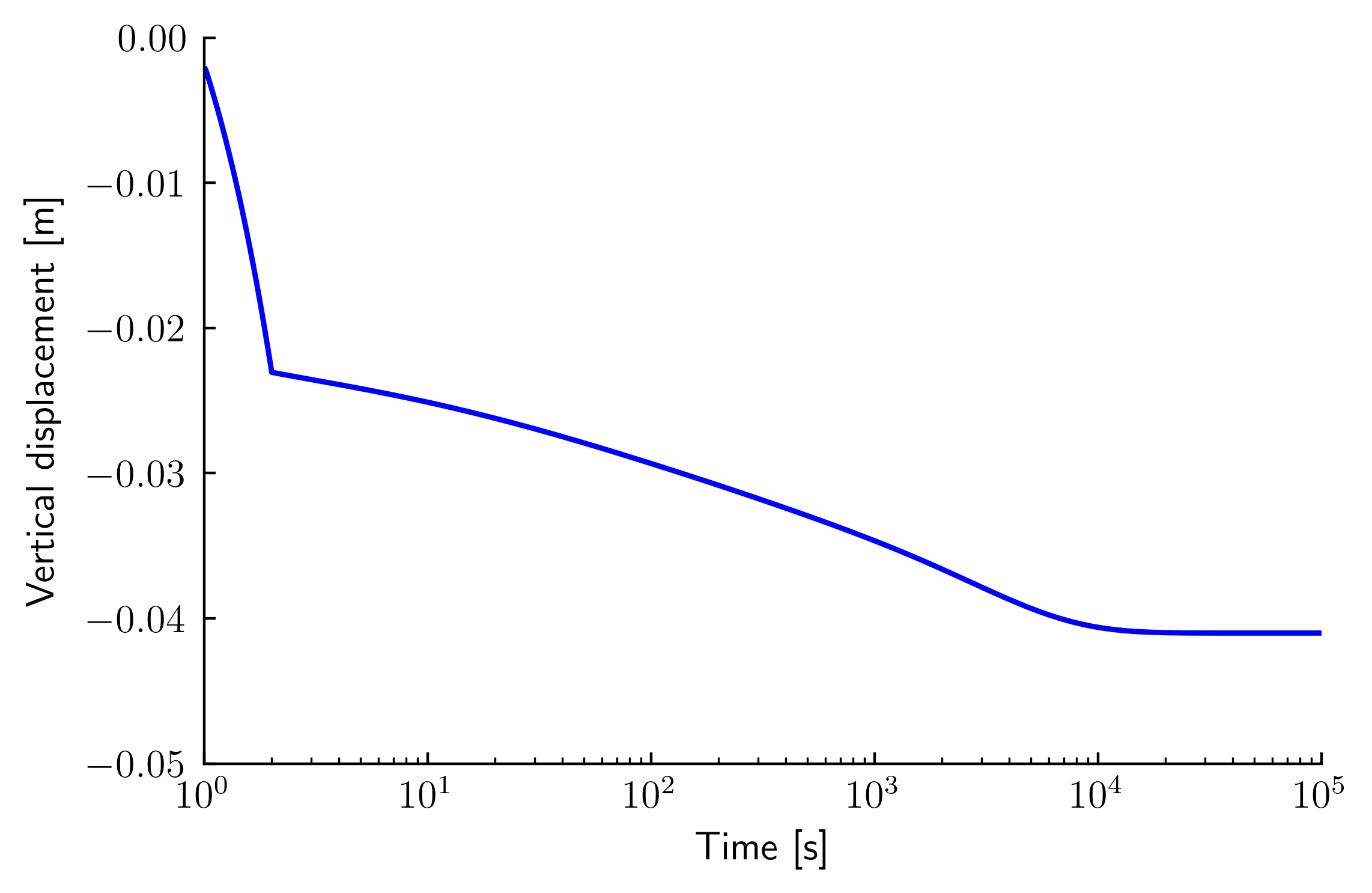Figure 2. Vertical displacement of the foundation

Python Script for plotting the results

The python script used to generate Figure 2 is given below:

import matplotlib
import matplotlib.pyplot as plt
import matplotlib.ticker as mtick
from pylab import genfromtxt
from matplotlib import rc
import os 
dir_path = os.path.dirname(os.path.realpath(__file__))
plt.rcParams['backend'] = "pdf"
plt.rcParams['xtick.direction'] = 'in'
plt.rcParams['ytick.direction'] = 'in'
plt.rcParams['text.usetex'] = True
plt.rcParams['font.size'] = 12
plt.rcParams['axes.spines.right'] = False
plt.rcParams['axes.spines.top'] = False
plt.rcParams['axes.linewidth'] = 0.8 

mylinewidth=1.6
mytextwidth=12

mat2 = genfromtxt(dir_path+'/input_foundation_soil_coupled-print-out/FOUNDATION.TOP_LEFT_NODE_node_7703.dat',skip_header=1);

plt.figure(1)
plt.subplot(111)

plt.semilogx(mat2[:,0], mat2[:,2],'b', linewidth=mylinewidth,\
         markersize=4,markerfacecolor='none',\
         clip_on=True,label=r"$k = 10^{-5}$ m/s")

ax = plt.gca()

ax.set_xlabel(r'Time [s]',fontsize=mytextwidth)
ax.set_ylabel(r'Vertical displacement [m]',fontsize=mytextwidth,labelpad=7)

ax.axis([1,1e5,-0.05,0])

ax.tick_params(axis='x',direction='in',pad=5,labelsize=mytextwidth)
ax.tick_params(axis='y',direction='in',pad=5,labelsize=mytextwidth)

fig = plt.gcf()  
fig.savefig('disp_coupled_elastic.pdf', dpi=400 , bbox_inches='tight')
fig.savefig('disp_coupled_elastic.png', dpi=400 , bbox_inches='tight')