1D infiltration (Srivastava & Yeh)
Analytical solution
An analytical solution for an 1D uncoupled transient infiltration problem into a soil proposed by Srivastava & Yeh (1991)1 is modelled. The solution includes exponential models for the relative permeability and water retention curves with total height \(l\), hydrostatic suction profile and infiltration via a rate $q_{inf} $:
The solution for \(\psi\) is proposed as:
$$ \psi = \frac{1}{\zeta} \cdot \ln{B}, $$ where as \(B\) is:
with
and wherein \(\lambda_i\) is the \(i^{th}\) root of the solution of the characteristic equation:
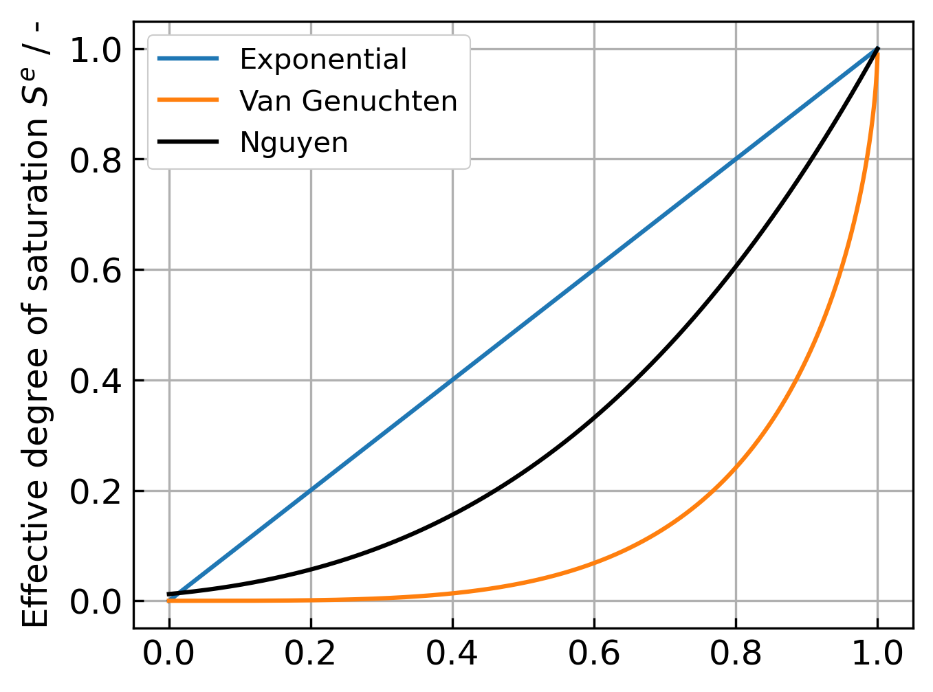
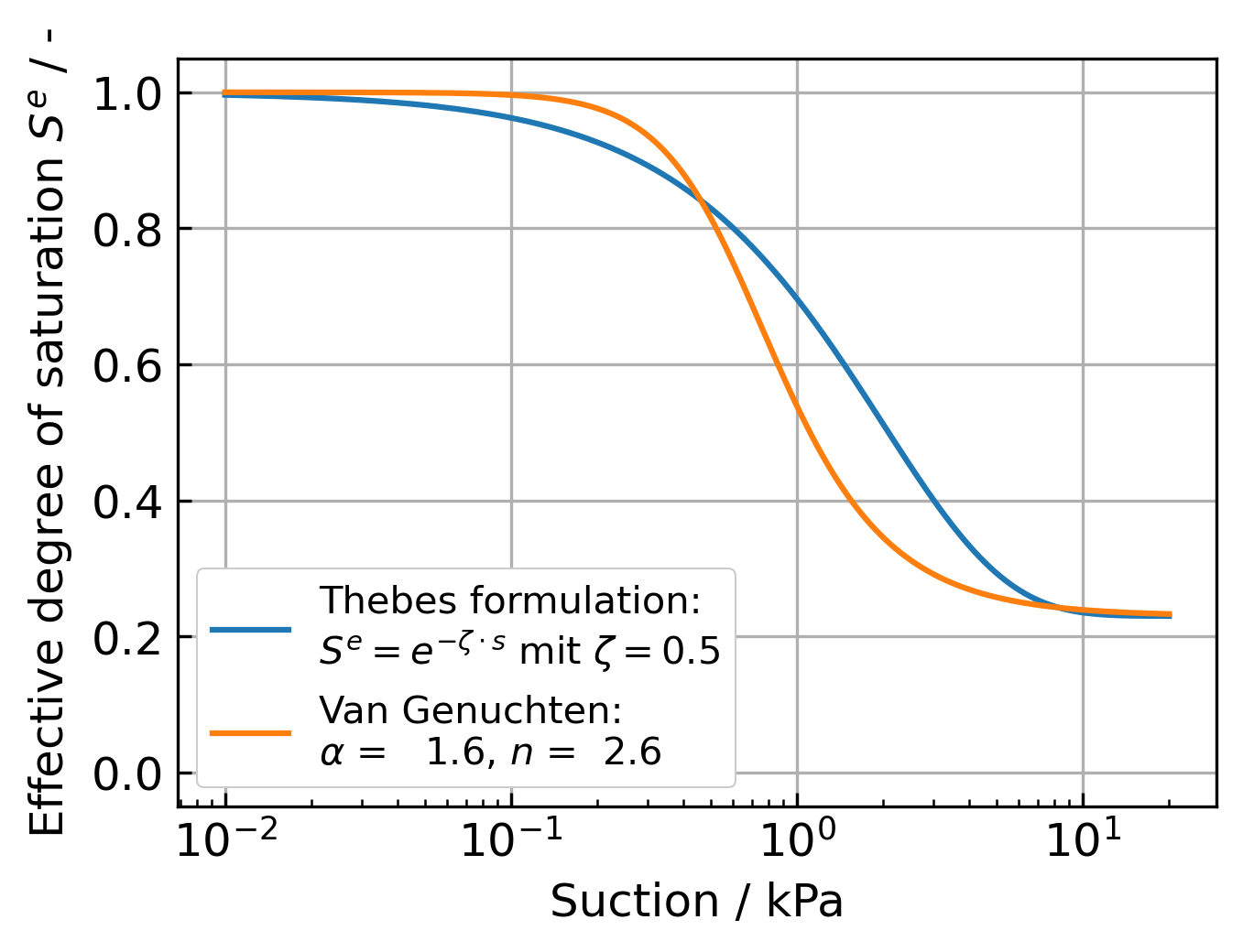
The exponential models for the relative permeability and water retention curve compared to more widely used approaches are visualised below:
numgeo simulation
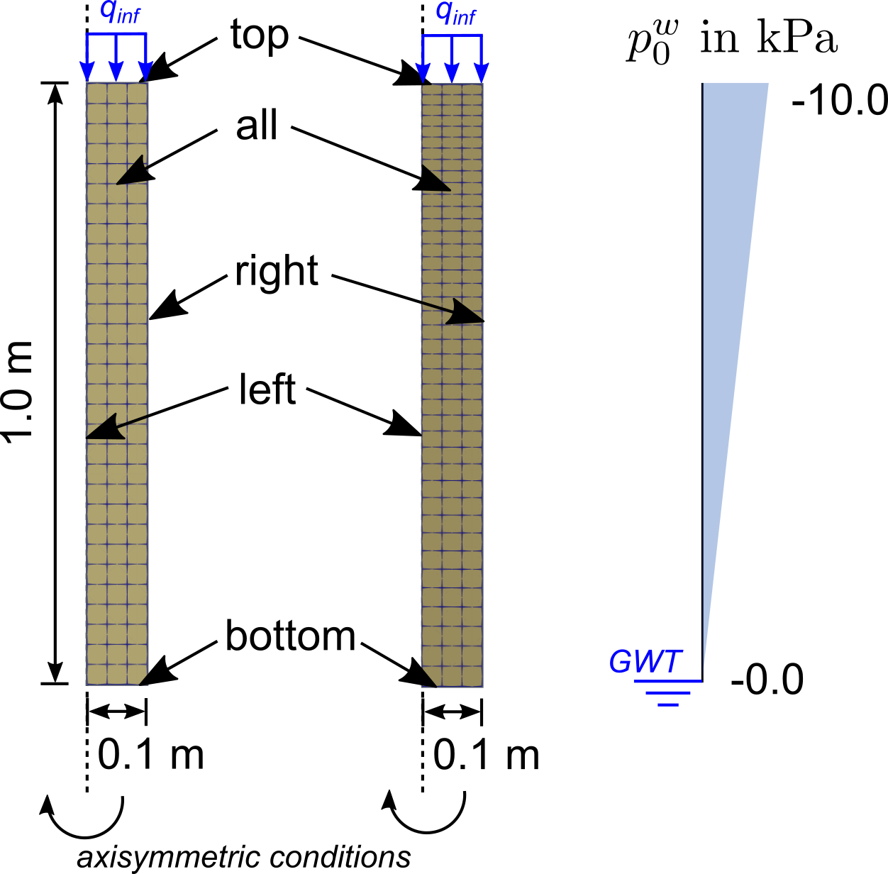
Model, boundary and initial conditions
The model definitions and initial conditions are shown below. An axisymmetric column is infiltrated by a flow boundary condition from the top andTwo meshes were used, one with quadratic elements (\(b=h=0.033\) m), and a second mesh where the element height increased gradiently from \(h=0.0165\) m to \(h=0.033\) m from top to bottom (discretizing the mesh finer where the infiltration takes place). Elements of type u8p4-ax were used (8-noded axisymmetric elements with quadratic interpolation). For this simulation, changes in pore air pressure are judged as negligible, thus elements based on reduced set of governing equations are used. These elements consider negative pore water pressures as suction \(s=-p^w\) (instead of \(s=p^a-p^w\)). The initial pore water pressure distribution \(p^w_0(z)\) is hydrostatic with the ground water table at the bottom of the column.
In general the analytical solution can be evaluated for different material parametes and initial conditions. For the validation with numgeo the following were chosen (following a validation by Abed & Solowksi (2017)2):
- \(K^l_{sat} = 0.1\) m/day \(= 1.157 \cdot 10^{-13}\) m\(^2\)
- \(\zeta = 5.0\) 1/m
- \(S^l_{res}=0.23\) and \(S^l_{sat}=1.0\)
- Geometry: \(h=l=1.0\) m and \(b=0.1\) m
- Ground water table in the bottom and infiltration rate \(q=0.005\) m/day \(= 5.787 \cdot 10^{-8}\) m/s
- Initial void ratio \(e_0 = 0.6667\)
Input files
The input files for the benchmark simulation can be downloaded here
Material
For the solid a linear elastic constitutive model is chosen. As no soil deformation is considered this choice is completely arbitrary. The Young's modulus is \(10 \cdot 10^5\) kPa and the Poisson's ratio \(0.4\).
Note that numgeo requires the prescription of the permeability \(K^s\) of the solid and the dynamic viscosity of the pore fluids \(\mu^f\) instead of the hydraulic conductivity \(K^f\), which are related as follows:
Therein, \(\gamma^f\) and \(\mu^f\) are the specific weight and the dynamic viscosity of the fluid \(f\), respectively.
The dynamic viscosity of pore water is \(\mu^w=10^{-6}\) kPa\(\cdot\)s and of the pore air \(\mu^a=10^{-8}\) kPa\(\cdot\)s. Assuming a specific weight of 10 kN/m\(^3\) for the pore water, the permeability of the soil is calculated to \(1.157 \cdot 10^{-13}\) m\(^2\).
Calculation stages
The simulation is divided into 2 steps in total: - During the Geostatic step, the self weight of the soil (grains and pore water) is applied without generating any deformation. As stated previously, no deformation of the soil skeleton is expected. We therefore constrain the displacements of all nodes in \(x1\) and \(x2\) direction. In addition, we use boundary conditions to prescribe the pore water pressure for each node assuming a hydrostatic distribution with the groundwater table described at \(z=0\) m:
*BOUNDARY,type=hydrostatic
nall,pw,-10.0d0,0.00d0
- During the transient step we simulate the water supply at top of the soil column. This is done by prescribing a flow boundary condition at the upper surface of the column with \(q=0.005\) m/day \(= 5.787 \cdot 10^{-8}\) m/s. Due to the strong nonlinearities resulting from the saturation-suction relation and the relative permeability function, we limit the maximum allowed time increment size to 500 seconds.
Results
The following figure presents the distribution of the pore water pressure over the column height for different time steps of the simulation. The comparison of the simulation results obtained with numgeo and the results of the analytical solution show an excellent agreement.
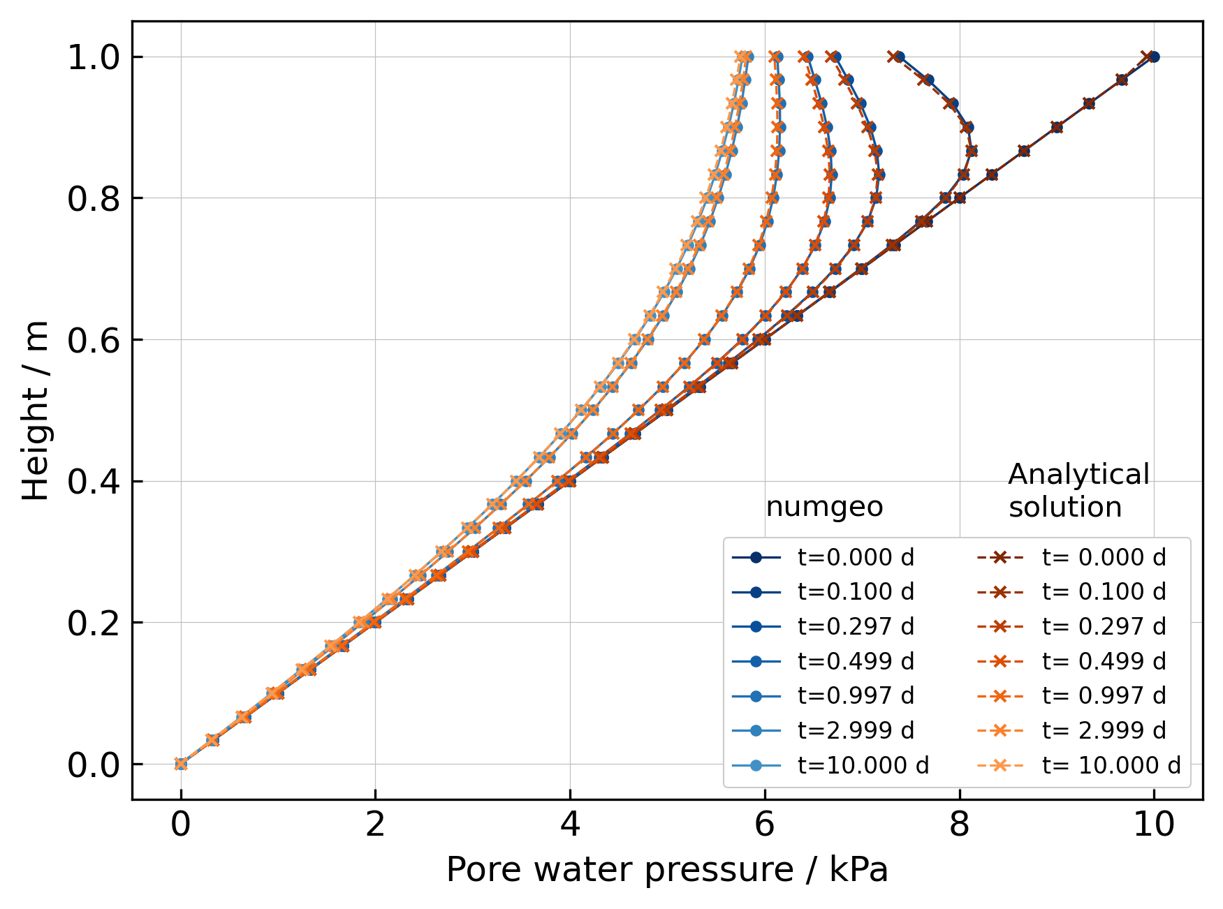
Distribution of degree of pore water pressure over the column height for different time steps of the simulation. numgeo vs. the analytical solution.
Automatic benchmarking results
This benchmark is part of an automated test suite executed before every software release to ensure the accuracy and reliability of the code. The following table shows the performance of the current numgeo release by comparing its results against a known analytical solution.
The metric used for comparison is the mean relative error, which quantifies the average deviation of the simulation from the exact analytical values. A lower mean error indicates a higher degree of accuracy for the given element type.
| u8p4 | u8p8-stab | p8 | u10p10-stab | u20p20-stab | u20p20-stab-red | u8p8-3d-stab | u8p8-3d-stab-red | |
|---|---|---|---|---|---|---|---|---|
| t = 0.0d | 0.02 % | 0.02 % | 0.02 % | 2.50 % | 2.50 % | 2.50 % | 2.50 % | 2.50 % |
| t = 0.1d | 0.08 % | 0.12 % | 0.09 % | 2.59 % | 2.62 % | 2.62 % | 2.60 % | 2.60 % |
| t = 0.3d | 0.10 % | 0.13 % | 0.12 % | 2.61 % | 2.62 % | 2.62 % | 2.61 % | 2.61 % |
| t = 0.5d | 0.12 % | 0.14 % | 0.12 % | 2.61 % | 2.63 % | 2.63 % | 2.62 % | 2.62 % |
| t = 1.0d | 0.13 % | 0.15 % | 0.13 % | 2.62 % | 2.63 % | 2.63 % | 2.63 % | 2.63 % |
| t = 3.0d | 0.14 % | 0.14 % | 0.12 % | 2.61 % | 2.62 % | 2.62 % | 2.63 % | 2.63 % |
| t = 10.0d | 0.15 % | 0.14 % | 0.12 % | 2.61 % | 2.61 % | 2.61 % | 2.63 % | 2.63 % |
| Overall (%) | 0.10 % | 0.12 % | 0.11 % | 2.59 % | 2.61 % | 2.61 % | 2.60 % | 2.60 % |
-
Srivastava, R. & Yeh, T.-C. J. Analytical solutions for one-dimensional, transient infiltration toward the water table in homogeneous and layered soils. Water Resour. Res., 1991, 27, 753-762. ↩
-
Abed, A. A. & Sołowski, W. T. A study on how to couple thermo-hydro-mechanical behaviour of unsaturated soils: Physical equations, numerical implementation and examples. Computers and Geotechnics, 2017, 92, 132-155. ↩