Dry elastic soil
The input files can be downloaded here.
Definitions in the input file
Open the previous created .inp file named \(input\_foundation\_soil\) using
a text editor, e.g. Notepad or Geany. After the statement
*Include = mesh_Foundation, add the node set \(top\_left\_node\):
*Instance, Name=Foundation, Part = Foundation
*Include = mesh_Foundation
*Nset, nset=top_left_node, find
0, 10.5, 0
*End Instance
This node will later be used for the output of the vertical settlement
of the foundation. It is defined by its geometrical position using the find option and located at the top left corner of the foundation. After the node set definition, add the following surface definitions:
**
** Surfaces
**

*Surface, type=node, name=surf_soil_top
Soil.top
*Surface, type=node, name=surf_foundation_bottom
Foundation.bottom
*Surface, type=node, name=surf_foundation_top
Foundation.top
Each surface definition contains an underlying node set. The node sets for the surface were generated by the python script used the in the mesh generation and can also be viewed in the input file.
Since two different materials are used, two separate sections have to be generated. The materials are defined in the next step:
**
** Material
**

*Material, name = soil, phases = 1
*Mechanical = Linear_Elasticity
10000, 0.3
*Density
2.0

*Material, name = foundation, phases = 1
*Mechanical = Linear_Elasticity
500000, 0.3
*Density
2.0
For the dry case, both materials are composed by just one phase. Both materials are assumed to behave elastically, using a Young's modulus of 10,000 kPa and a Poisson's ratio of 0.3 for the soil and 500,000 kPa and 0.3 for the foundation. Both have a density of 2 g/cm\(^3\).
The contact conditions are defined in the following:
**
** Contact
**

*Interaction, name = penalty, mechanical=Penalty, no separation
*friction, model= MC
0.2,0,0
*Contact Pair, interaction = penalty, discretisation = element mortar
surf_soil_top, surf_foundation_bottom
The previously defined interaction is used in a Contact Pair
definition. A contact pair is a set of surfaces constrained by the
defined interaction and discretised by the chosen discretisation. In
the present case, a mortar discretisation is used. The contact
discretisation is used to evaluate the contact distance, compute the
contact quantities and integrate the contact contributions to the
overall system of equations. Friction is considered by a simple Coulomb friction model with a friction coefficient of \(\mu = 0.2\).
The initial stress state is defined as \(K_0\) stress state using:
**
** Initial conditions
**

*Initial conditions, type = stress, geostatic
Soil.all, 10, 0, 0, -200, 0.5, 0.5
Therein the element set \(Soil.all\) is assigned an initial stress state with \(\sigma_2(y=10.0\) m\()=0.0\) kPa and \(\sigma_2(y=0.0\) m\()=-200\) kPa (\(\gamma =20\) kN/m\(^3\)). \(K_0\) is 0.5 in x as well as in z direction.
For the analysis, time variations of boundary and loading conditions have to be defined. This is done using the following amplitude definition:
**
** Amplitudes
**

*Amplitude, name = LoadingRamp, type = ramp
0.0, 0.0, 1.0, 1.0
The amplitude \(LoadingRamp\) defines a linear increase of a quantity beginning with the relative value 0 at the time \(t_1=0\) and the relative value 1 at the time \(t_2=1\).
The first step of a geotechnical analysis is usually the so called
Geostatic step wherein the initial stress state is checked against the
stress state resulting out of gravity. An initial stress state that is
not in accordance with the gravitational stress state eventually leads
to displacements. In general, the smaller the displacement after the
Geostatic step, the better the stress state accords the stress due to
gravity. Too large values of displacement indicate a falsification of
the initial state that is crucial in case of path dependent constitutive
models such as the hypoplasticity.
First, the step environment has to be started by the keyword *Step and the name of the step has to be defined. The
analysis type of the step is given in line 2, which will be a Geostatic
step. The keyword Body force imposes a gravitational force which is
applied instantaneous (instant). The element sets \(Soil.all\) and
\(Foundation.all\) are loaded by the gravity (amplitude \(9.99\) m/\(s^2\),
directed downwards with the normalized vector of the gravity
\(\vec{\textbf{b}}=\{0,-1,0\}\)).
**
** Load step 1
**

*Step, name=step1, inc = 1
*Geostatic

*Body force, instant
Soil.all, GRAV, 9.99, 0, -1, 0
*Body force, instant
Foundation.all, GRAV, 9.99, 0, -1, 0
Following the definition of the loads, the Dirichlet boundary conditions are specified. All nodes of the foundation are constraint in 1- as well as in 2-direction in the Geostatic step. Therefore, no displacement of the foundation is possible. The soil area is only constrained at the bottom in vertical direction and at both lateral sides in horizontal direction.
*Boundary
Foundation.all,u1, 0.0d0
Foundation.all,u2,0.0d0
Soil.left,u1,0.0d0
Soil.right,u1,0.0d0
Soil.bottom,u2,0.0d0
The output is written in the vtk format (suitable for ParaView) and is
of ASCII type. The node output includes the displacement (U) of the
nodes and the element output includes the stress (S) as well as the
contact output variables (Contact). The contact output contains of
contact stresses as well as of contact distances for each contact node. Finally, the step environment is closed by the keyword *End step.
*output, field, vtk, ASCII
*node output, nset = Soil.all
U
*element output, elset = Soil.all
S, Contact

*End Step
In the second step, the foundation is released and loaded. A static analysis type is chosen, where an incrementation scheme as given in line 3 is used. The initial increment is 0.01, the total step time is 1, the minimum allowed increment is 0.0001 and the maximum increment is 0.01. Note that time does not correspond to physical time in a static step but rather is the fraction of an applied load or boundary condition. The static analysis type indicates that no inertia forces (and therefore no physical time dependencies) are considered.
**
** Load step 2
**

*Step, name=step2, inc = 10000
*Static
0.01,1.0,0.0001,0.01
In numgeo, previous imposed loads have to be redefined in every
subsequent step in which they are supposed to be active. Therefore, the
gravity is applied again.
*Body force, instant
Soil.all, GRAV, 9.99, 0, -1, 0
*Body force, instant
Foundation.all, GRAV, 9.99, 0, -1, 0
The boundary conditions for the soil remain the same as in the first step but the foundation is now only constrained horizontally in the symmetry axis. The foundation is now free to penetrate into the soil vertically.
*Boundary
Foundation.left, u1, 0.0d0
Soil.left,u1,0.0d0
Soil.right,u1,0.0d0
Soil.bottom,u2,0.0d0
The top of the foundation is loaded up to 500 kPa linearly increasing over
the step time using the previously defined amplitude. Alternatively, instead of specifying amplitude = LoadingRamp, ramp could be used, which automatically linearly increases a quantity over the step duration.
*DSload, amplitude = LoadingRamp
surf_foundation_top, p, -500.0d0
The "global" convergence controls are disabled and only the local convergence criteria are active. The field output remains indentical to the 1. step. A print output is added, which produces a separate output folder named "print-output". In this folder, the requested variables are written for the requested node or element sets with respect to the step time. This enables the results of individual nodes, elements or sets of nodes/elements to be conveniently plotted. The *frequency statement allows to control the frequency with which the print output is written with respect to the increments of the step. Finally, the step is closed with *End Step and the input file with *End Input.
*Controls, global, deactivate
*Controls, u, activate

*Output, field, vtk, ASCII
*Node output, nset = Soil.all
U
*Element output, elset = Soil.all
S, Contact

*Output,print
*frequency = 1
*Node output, nset = Foundation.top_left_node
U

*End Step

*End Input
Results of the simulation
After the calculation is finished (the command window is ready for a new command), open the .sta file first and check that the simulation was successful by identifying that both steps have been completed successfully. If the calculation immediately stops, check the error message in the .log file. The progress of the simulation can also be checked during the analysis by opening the .sta file.
To see the output of a step, start ParaView and open the pvd file (in
the right upper options bar: "File" \(\rightarrow\) "Open...") that
is present in the calculation folder.
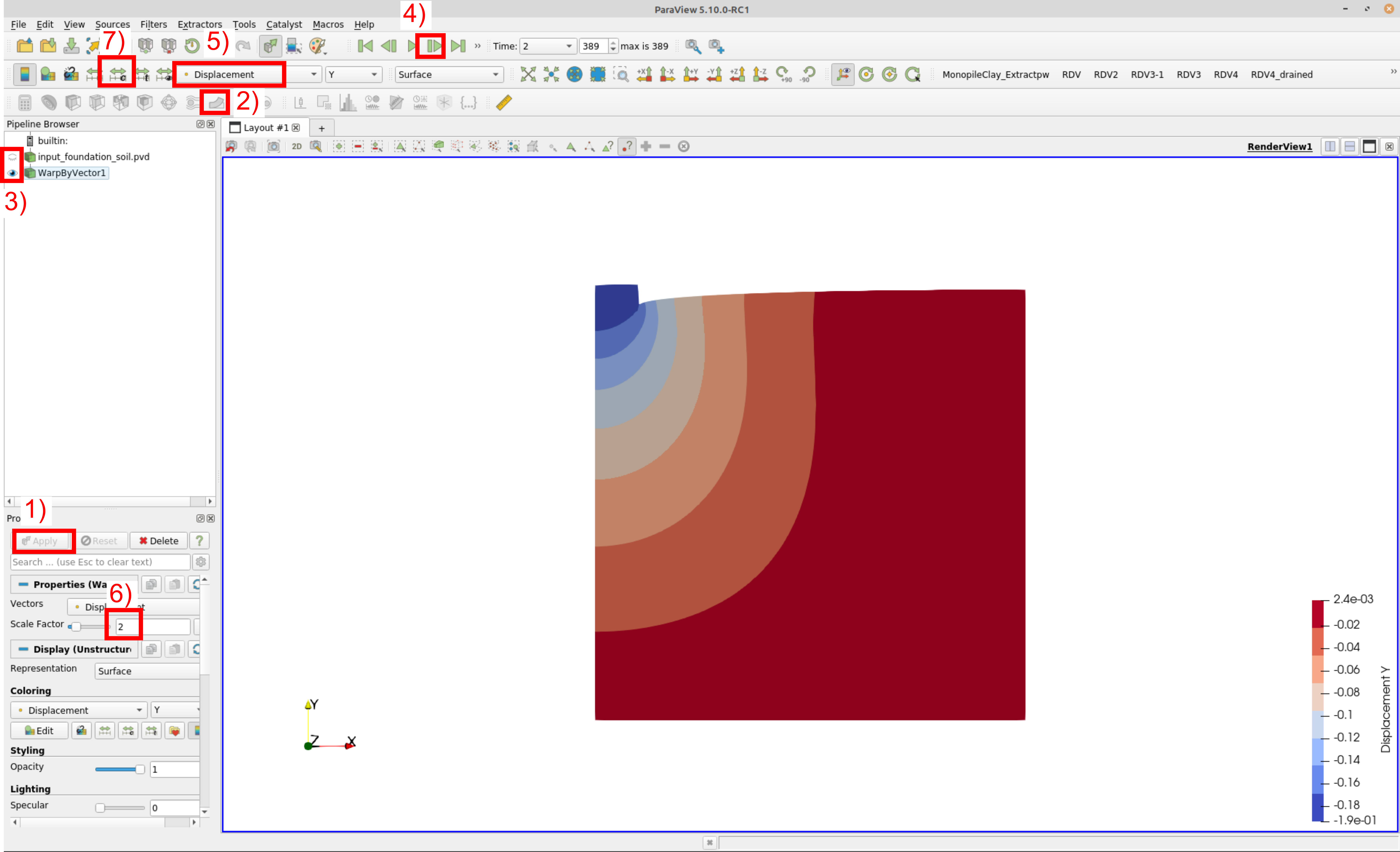 Figure 1. Vertical displacement at the end of the second step
To display the deformed system at the end of the second step, follow the steps shown in Figure 1. Note that in (step 6) a deformation scale factor of 2 is chosen. This means that the deformed state is depicted with 2 times greater displacement.