Slope with random field
Quick read on strength-reduction analysis
The strength reduction method is a separate calculation type that can be selected using the keyword *Reduction in the step definition. During a strength reduction analysis, the shear strength parameters of the soil are incrementally reduced in accordance with a strength reduction factor (SRF) until failure is obtained. The SRF is applied to the tangent of the friction angle and the cohesion to ensure equal proportion of shear resistances by frictional and cohesive terms throughout the strength reduction. Assuming that the factor of safety (FoS) is identical to the SRF, the reduced shear strength parameters \(\varphi_\text{red}\) and \(c_\text{red}\) can be determined based on the actual shear strength parameters and the FoS as follows:
\(\tan \varphi_\text{red} = \tan \varphi\,/\,\text{FoS} \qquad \text{and} \qquad c_\text{red} = c\,/\,\text{FoS}\)
To control the incremental reduction of the shear strength parameters, the line following the keyword *Reduction requires the definition of four scalars: an initial value of the factor of safety (FoS\(_0\)) and an initial step-size (\(\Delta\)FoS\(_0\)), a maximum step-size (\(\Delta\)FoS\(_{\max}\)) and a minimum step-size (\(\Delta\)FoS\(_{\min}\)) need to be prescribed in the calculation type definition. During a strength reduction analysis, FoS is incrementally increased, which results in an incremental reduction of the shear strength parameters.
The strength reduction method can be used in combination with the Mohr-Coulomb and Matsuoka-Nakai model, so far. To specify that the shear strength parameters of a specific material parameter set should be reduced during a strength reduction analysis, the keyword *Reducible Strength needs to be specified in the material definition.
Detection of failure is conducted based on non-convergence. Moreover, post-processing can be used additionally to inspect the maximum displacements vs. FoS. Plotting the former in logarithmic scale, slope failure can also be defined as the FoS associated to a decisive kink in the curve trend.
The aim of this tutorial is to show how the concept of Random Fields can be coupled with a strength-reduction analysis in numgeo. For the sake of brevity we will consider the same finite element model used in the tutorial on the Homogeneous slope and originally presented by Pruška (2009)1. This homogeneous slope has a height of 7 m and a width of 10 m and is shown in Figure 1.
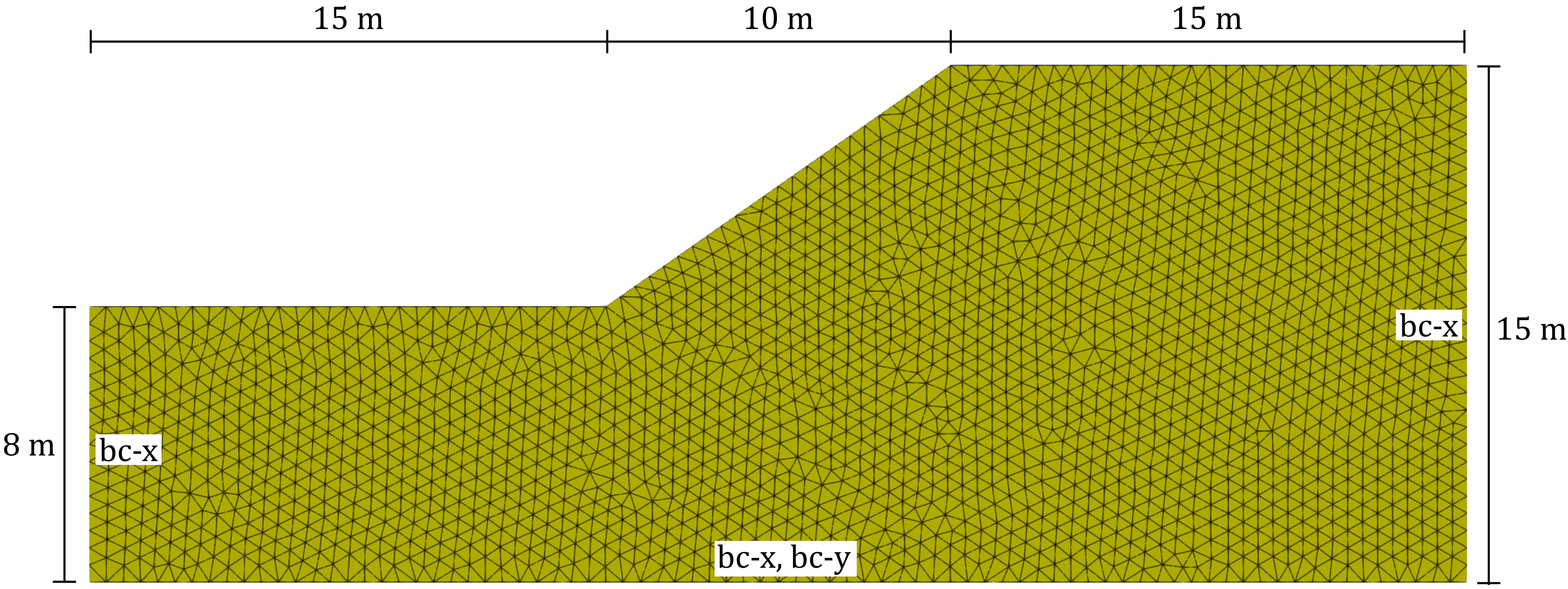
Figure 1. Problem setting and representative finite element mesh of the homogeneous slope used in this tutorial.
The linear elastic, perfectly plastic Mohr-Coulomb (M-C) model is used in the analysis. Contrary to the previous tutorials we will consider spatial variations in effective friction angle \(\varphi\) and effective cohesion \(c\). The spatially varying fields have been created with a Random Field tool developed at TU Darmstadt. The random fields were created using Gaussian correlation functions with assumed mean values of \(\bar{\varphi}=25^\circ\) and \(\bar{c}=10\) kPa and coefficients of variations of \(cov^{\varphi}=0.1\) and \(cov^{c}=0.3\). The correlation lengths are assumed to be 30 m and 10 m in the horizontal directions and 2 m in vertical direction. The friction angle and the effective cohesion are negatively correlated with a correlation coefficient of -0.5. One representative random field generated with these settings is shown in Figure 2. The data of these fields is provided as tabular data in the text files rf_phi_3.txt and rf_c_3.txt in the supporting files of this tutorial.
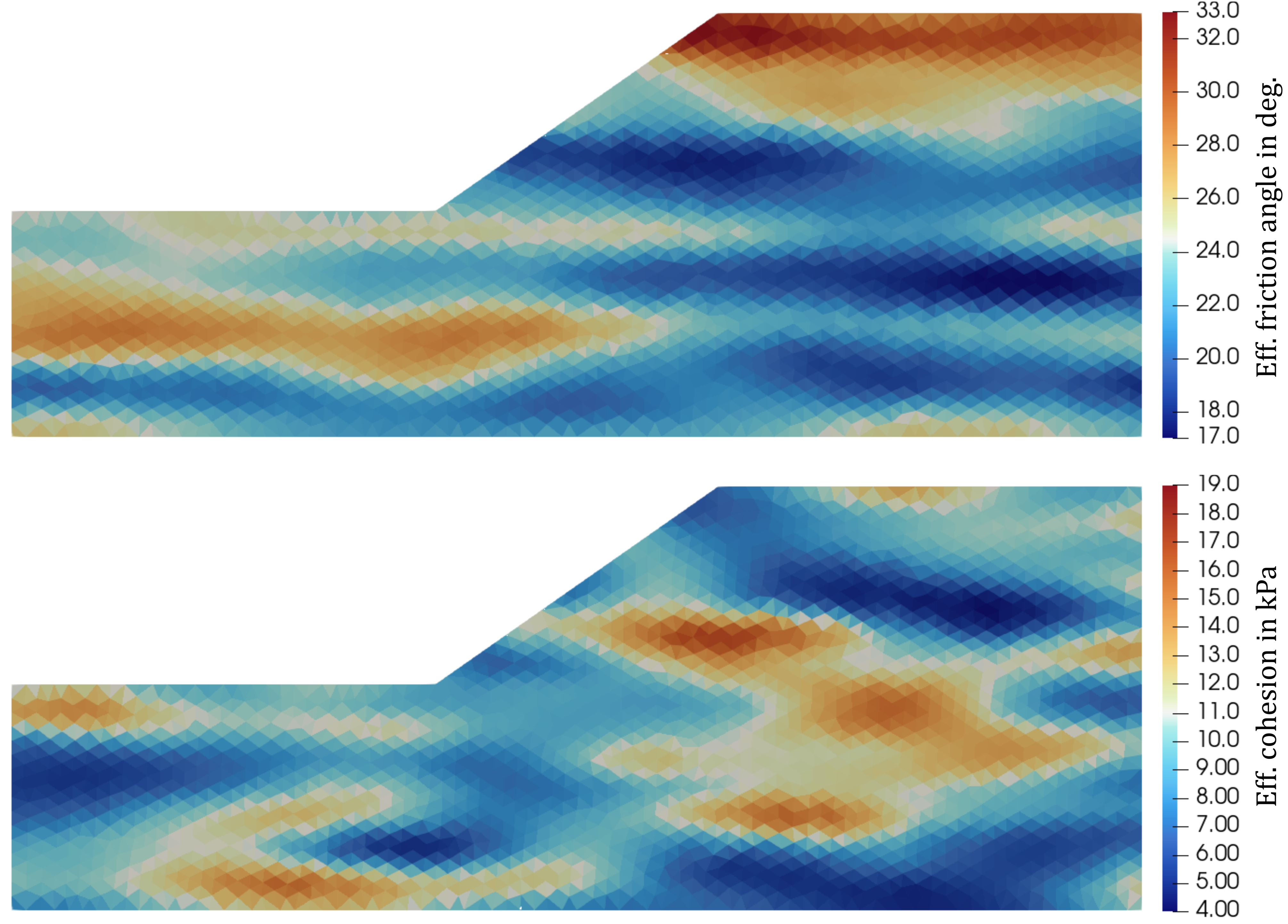
Figure 2. Spatially varying fields of effective friction angle and effective cohesion.
Notice that the graphical representation of the random fields displays mean values of the actual integration points of the elements. The actual random field is smoother as displayed in Figure 2. The remaining parameters of the Mohr-Coulomb model are assumed as follows: Young's modulus \(E=5000\) kPa, Poisson's ratio \(\nu=0.3\) and dilatation angle \(\psi=0.01^\circ\). The density of the soil is \(\rho=2.4\) (t/m³). A tension cut-off of \(p_t=0\) kPa is used.
Input files
The input files for the tutorial can be downloaded here.
Finite element mesh
The finite element model was created using the GiD pre-processing software, the corresponding GiD (GUI) files from here. For the discretisation of the domain, two-dimensional u-solid finite elements are used, discretising the displacement (u) of the solid. The mesh is composed of 6-noded triangular elements with quadratic interpolation order (termed u6-solid).
.
.
*Element, Type = U6-solid
.
.
In the mesh file, node sets (NSet) and element sets (ElSet) have been defined to address groups of nodes and elements to be used in the step files (e.g. for the definition of boundary conditions). The following node sets have been defined in the mesh file and used in the step files: bc-x, bc-y, all. Only one element set has been defined: all. For bc-x and bc-y see also Figure 1
To keep the input file as short as possible, we store the finite element mesh in a separate file pruska-2009-rf-mesh.inp and import it at the beginning of the actual input file pruska-2009-rf.inp containing the material and calculation specifications:
*Include = pruska-2009-rf-mesh
Material definition
The material parameters are chosen as described in the introduction of this tutorial and follows a similar procedure as in the previous tutorials on strength reduction analyses.
To consider that shear strength parameters of a specific material parameter set should be reduced in a strength reduction analysis, the keyword *Reducible Strength needs to be specified in the material definition.
New in this tutorial is the consideration of spatially varying friction angle and cohesion via random fields. However, the *Material keyword does not allow to assign multiple values, or even spatially varying values, of material parameters. The approach for random fields implemented in numgeo is as follows:
-
Define the material as you would in a standard simulation using dummy values for the random field parameters. In this case the dummy values are \(\varphi=30^\circ\) and \(c=0.1\) kPa. All other parameters, e.g. \(E\) or \(\rho\), are the actual parameters of the material.
*Material, name=case1, phases=1 *Mechanical = Mohr-Coulomb-2 5000, 0.3, 0.1, 30, 0.0, 0 *Density 2.4 *Reducible Strength -
Use the
*Initial condition, type = state variablekeyword to import the spatially varying fields of friction angle and cohesion. Details follow in the next section.
Initial conditions
In this example we will start the simulation from a stress-free and gravity-free state and slowly increasing the gravity to establish the initial stress field. Thus no initial stress is prescribed.
However, as already mentioned in the previous section, we will use the *Initial condition, type = state variable keyword to import the spatially varying fields of friction angle fric and cohesion coh. The Mohr-Coulomb-2 implementation allows to override the values given for \(\varphi\), \(c\) and \(\psi\) in the *Material definition at integration point level.
In the present example these spatially varying fields are provided by means of tabular data in text files (rf_phi_3.txt, rf_c_3.txt). The command for import of the data reads as follows:
*initial conditions, type=state variables, xy-data
all, fric, rf_phi_3.txt
*initial conditions, type=state variables, xy-data
all, coh, rf_c_3.txt
The keyword xy-data tells numgeo that the data is provided in terms of a series of spatial points with x- and y-coordinates and associated values for the friction angle fric and cohesion coh, respectively. Exemplarily, the first lines of the file rf_phi_3.txt are given below.
npoints, 12078
 X1 X2 phi
8.33333e-02 3.33333e-01 2.63839e+01
8.33333e-02 8.33333e-02 2.64218e+01
3.33333e-01 8.33333e-02 2.64165e+01
8.34140e-02 8.67335e-01 2.34682e+01
... ... ...
The assignment of the data to the integration points is performed by numgeo by means of a nearest neighbour search. More information on the different options to import spatially varying fields from text files is given in the Reference manual. The resulting fields are shown in Figure 2.
Amplitudes
Amplitudes need to be defined to allow for changes of loads or boundary conditions during a step. For this example, only a simple loading ramp is needed to incrementally increase the gravity during the first loading step
*Amplitude, Name=loading, Type=ramp
0, 0, 1, 1
Steps
The simulation consists of a total of two steps. During the first step, the gravity is increased starting from 0 m/s² to 10 m/s². In the second step, the strength-reduction is performed to estimate the safety of the system against failure.
Step 1
The gravity increase is performed assuming quasi-static conditions (*Static)
*Step, name=Step 1, inc=1e4, maxiter=32, miniter=1
*Static
0.01, 1, 0.001, 0.1
The displacements of the lateral model boundaries are constrained in horizontal directions, the displacements at the base of the model are constrained in vertical and horizontal direction.
*Solver, Pardiso
*Boundary
bc-x, u1, 0
*Boundary
bc-y, u2, 0
The gravity is increased from its initial value of 0 m/s² to 10 m/s² following a linear relation with the step time:
*Body force, amplitude=loading
all, Grav, 10, 0.0,-1.0,0.0
Finally, we specify the output. In this case, we want to display the simulation results in Paraview. Specifically, we are interested in the displacements u, the stress s and the strain e as well as the friction angle fric and cohesion coh:
*output, field, VTK, ASCII
*frequency=1
*node output, nset = all
u, s, e
*element output, elset = all
s, e, fric, coh
Lastly we close the step:
*End Step
Step 2
In the second step we perform the strength reduction simulation. With the keyword *Reduction, numgeo uses an automatic procedure to determine the Factor of Safety (FoS) for the current system by incrementally decreasing (and increasing) the shear strength parameters.
*Step, name=Step 2, inc=1e4, maxiter=16, miniter=1
*Reduction
0.95, 0.05, 0.05, 1e-4
*Extrapolation, FoS-linear
The boundary conditions remain unchanged:
*Boundary
bc-x, u1, 0
*Boundary
bc-y, u2, 0
The increase in gravity performed in the first step leads to significant deformations in the system. These are not of relevance for the stability analysis but might render the interpretation of the results more difficult. We thus reset the displacements and strains:
*Reset
Displacement, Strain
The gravity now acts as a constant load
*Body force, instant
all, Grav, 10, 0.0,-1.0,0.0
we further help the newton iterations by enabling the Anderson accelerator of depth 2:
*Accelerator, type=anderson
2, 2
and we add the Factor of Safety (FoS) to the output request:
*Output, field, VTK, ASCII
*frequency=1
*node output, nset = all
u, S, e,  FoS
*element output, elset = all
s, e, fric, coh
Finally, we end the step
*End Step
and close the input file:
*End Input
Results
The displacement contour plot and deformed geometry at failure are depicted in Figure 3. The simulation results show a clear failure mechanism resembling a shallow circular slip surface.
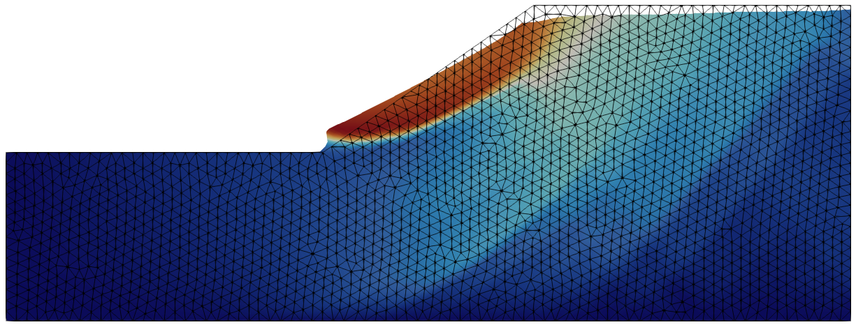
Figure 3. Displacement contour plot and deformed geometry at failure (magnification x10).
The evolution of the Factor of Safety (FoS) vs. the maximum displacement magnitude is displayed in Figure 4. The final FoS is 1.183.
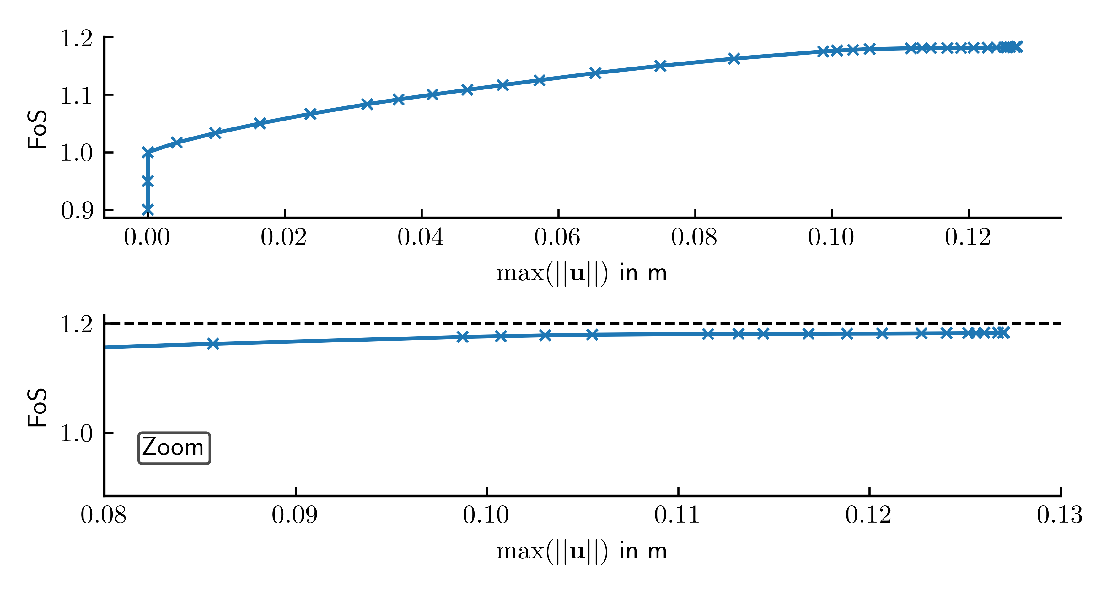
Figure 4. Max. displacement magnitude versus Factor of Safety (FoS).
The python script used to produce this plot is given below. The FoS, max. displacement and internal energy data plotted in Figure 4 is saved as an output automatically by numgeo at the end of a strength-reduction analysis and saved in a csv file, here named step2-strength-reduction-history.csv.
#%%
import numpy as np
import matplotlib.pyplot as plt

fontsize = 10
plt.rcParams['xtick.direction'] = 'in'
plt.rcParams['ytick.direction'] = 'in'
plt.rcParams['text.usetex'] = True
plt.rcParams['font.size'] = fontsize
plt.rcParams['axes.spines.right'] = False
plt.rcParams['axes.spines.top'] = False
plt.rcParams['axes.linewidth'] = 1.0

# Convert centimeters to inches for figure sizing
def cm2inch(*tupl):
    inch = 2.54
    if isinstance(tupl[0], tuple):
        return tuple(i/inch for i in tupl[0])
    else:
        return tuple(i/inch for i in tupl)


data = np.genfromtxt('./step2-strength-reduction-history.csv', delimiter=',', skip_header=1)

fig, ax = plt.subplots(2,1, figsize=cm2inch(15,8), sharex=False)

ax[0].plot(data[:,1], data[:,0], marker='x', markersize=4)
ax[0].set_xlabel('$\max(||\mathbf{u}||)$ in m')
ax[0].set_ylabel('FoS')
ax[0].set_yticks([0.9,1,1.1,1.2])

ax[1].plot(data[:,1], data[:,0], marker='x', markersize=4)
ax[1].hlines(1.2, 0.0, 0.13, color='k', ls='--', lw=1.)
ax[1].set_xlabel('$\max(||\mathbf{u}||)$ in m')
ax[1].set_xlim(0.08,0.13)
ax[1].annotate('Zoom', [0.082,0.96],
             bbox=dict(boxstyle="round,pad=0.15", edgecolor='k', facecolor='w', alpha=0.7))
ax[1].set_ylabel('FoS')

plt.tight_layout()

plt.savefig('./pruska-2009-rf-fos.png', dpi=600)
-
J Pruška. Comparison of geotechnic softwares-geo fem, plaxis, z-soil. Vanícek, et al., Eds., XIII ECSMGE, 2009. ↩