Vibratory pile driving in water-saturated sand
The input files can be downloaded here.
In this series the simulation of vibratory pile driving in water-saturated sand according to the simulations reported in1 is explained. The input file shipped together with this document and further described in the following is identical to the one used in1 from a technical point of view. Note that the input files used in2 are very similar to the one explained in this document.
All information about the numerical model used for the analysis can be obtained from1. This document only explains the definitions in the input file and not the general set-up of the numerical model.
Input file
The input file is split into two files: the mesh (mesh.inp) and the step file (step.inp). First, the mesh file is briefly explained.
Mesh file
u8-solid-ax elements are used for the pile and the unbalances, which
are placed on top of the pile and are connected to it by spring
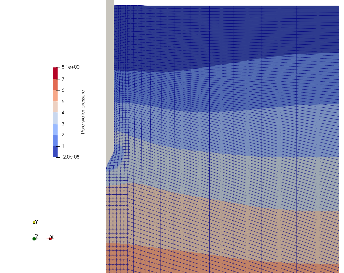
elements. For the soil, axisymmetric u-p finite elements with 8
nodes discretising the displacement u of the solid phase and 4 nodes
discretising the pore water pressure \(p^w\) are utilised (termed
u8p4-sat-ax-red element). A reduced integration scheme with 4
integration points is adopted. The corresponding definition can be found
in line 7550 of mesh.inp.
.
.
*Element, type=u8p4-sat-ax-red
.
.
Hence, quadratic interpolation functions are used for the solid displacement while linear interpolation functions are applied for the pore water pressure (i.e. Taylor-Hood element formulation3).
Properties, initial conditions and step definitions (Step file)
The step file (step.inp) first includes the mesh file by defining:
*include = mesh
In the model test by J. Vogelsang4, two pore water pressure transducers recorded the development of pore water pressure at different spatial positions during driving. In order to compare the measurements with the results of the simulations, the pore water pressure is also recorded in the numerical analysis. The points are defined by specifying their spatial position:
*nset, find, nset = top_pw
0.0386,0.6,0.0

*nset, find, nset = bottom_pw
0.025,0.35,0.0
The penalty method is used to enforce the contact constraints. No separation between soil and pile is possible once the contact is active. The penalty factor is \(3\cdot 10^6\) kN/m\(^3\). A simple Coulomb friction model is adopted, which properties are defined in a user-file, which is explained later in this Section. The contact between soil and pile is discretised using the element-based mortar contact discretisation technique, which implementation is discussed in detail in 5. A small value for the contact clearance is defined, which leads to a small value of initial contact pressure. This is beneficial since the initial stress state is closer to equilibrium, in which the earth pressure is acting as contact pressure.
*interaction, name = penalty, mechanical = penalty, no separation, user
5d6
*friction, model = mc
*contact pair, interaction = penalty, discretisation = element mortar
soil_pile_all, pile_soil_all
*contact options, name = penalty, clearance = 2d-5
Then the definitions of the solid sections and material definitions are given. The soil is modelled with the material hypo_soil while pile and unbalance are modelled elastically. However, the elastic properties are set arbitrarily high since no self-deformations occurred in the tests. Pile and unbalance also don't have a density, since their self-weight and inertia will be applied by concentrated forces and mass points, respectively.
*solid section, elset = soil_all, material = hypo_soil
*solid section, elset = pile_all, material = elastic
*solid section, elset = unbalance,  material = elastic

*material, name = elastic, phases = 1
*mechanical = linear_elasticity
5d10, 0.0
*density
1d-10
Only the hypoplastic model with intergranular strain extension is considered here as constitutive model for the soil. The input file for the simulations using Sanisand is easily obtained by replacing the following definitions. The parameters of the hypoplastic model with intergranular strain extension according to 1 are given below.
An artificial viscosity is used to achieve better convergence. The adopted values are further described in 1. To avoid positive mean effective stresses (in mechanical sign convention), a minimum value is set.
Two densities have to be given which are the density of the solid grains
and the density of water. In addition, the bulk modulus of the pore
water and the permeability have to be defined. In numgeo, the
permeability equals the dynamic viscosity (set to \(10^{-6}\) kPas)
multiplied with the hydraulic conductivity \(k^w\) and divided by the unit
weight of water (\(\gamma_w = 10~\)kN/m\(^3\)). As explained in
1 (and further evaluated in 2 ) the
Kozeny-Carman relation is used to consider the influence of the porosity
on the permeability.
*material, name = hypo_soil, phases = 2
*mechanical = hypoplasticity
0.577, 0.0, 19d6, 0.285, 0.549, 0.851, 1.15, 0.1
0.32, 1.2, 2.4, 5d-5, 0.08, 7, 0.

*mechanical viscosity = linear
0.5, 2.0, 0.1, 1, 0.1, 1
*minpressure
-0.01

*density
2.65, 1.0

*bulk modulus
1.2d4
*permeability = kozeny-carman
308, 0.5d-3
*dynamicviscosity
1.0d-6
The initial conditions for the state variables are defined in user subroutines (see the files shipped with this document and the explanations given later in Section. The void ratio used for the calculation of the density of the soil is given in line 3. This value does not necessary have to coincide with the value given in the user initial state file. The initial stresses according to the values given in 1 are defined. A hydrostatic pore water pressure is defined for the entire soil mass.
*initial conditions, type = void ratio, default
soil_all, 0.637

*initial conditions, type = state variables, user
soil_all

*initial conditions, type = stress, geostatic
soil_all, 0.81, -0.1, 0, -8.266, 0.455, 0.455
pile_all, 1, 0, 0, 0, 0.5, 0.50
unbalance, 1, 0, 0, 0, 0.5, 0.50

*initial conditions, type = pore water pressure, default
soil_all, 0.0, 8.1, 0.81, 0.0
For the analysis, different time distributions of boundary and loading conditions have to be defined. This is done using the following amplitude definitions:
*amplitude, name = loadingramp , type = ramp
0.0, 0.3, 1.0, 1.00

*amplitude, name = risingsine , type = rising_sine
0.075, 157.0, 1.0
The amplitude \(loadingramp\) defines a linear increase of a quantity beginning with the relative value 0.3 at the time \(t_1=0\) and the relative value 1 at the time \(t_2=1\). To apply the cyclic loading by the unbalances, a sinusoidal amplitude with a frequency of 25 Hz is defined in addition. For this amplitude, a linear increase for the first 0.075 s is assumed, considering that in the model tests, the unbalances also required a short time to achieve the targeted frequency.
Steps and loading definitions
The first step will be a geostatic step considering non-linear
geometry effects (nlgeom). The keyword Body force imposes a
gravitational force which is applied instantaneous (Instant). The
element set \(soil\_all\) is loaded by the gravity (Amplitude \(10\)
m/s\(^2\), directed downwards with the normalized vector of the gravity
\(\vec{\textbf{b}}=\{0,-1,0\}\)).
All nodes of the pile, unbalance and the soil are constraint in 1- and 2-direction
(i.e. radial and vertical direction). Therefore, no displacement is
possible for any node in the model. The pore water pressure is
prescribed hydrostatically using a boundary condition of type
hydrostatic. A small stabilising pressure of 0.1 kPa is applied at the
top surface of the soil.
Not active in the step but already being defined for the next step is a connector element, which connects unbalances and pile. The connector element mimics the spring between unbalances and pile used to measure the force. The spring stiffness is 173000 kN/m.
The output is written in the vtk format (suitable for ParaView) and is of ASCII
type. The node output includes the displacement (u) and pore water
pressure (pw) of the nodes. The element output includes the stress
(s), strain (e) as well as the void ratio (void_ratio) and the
contact output variables (contact). The contact output contains
contact stresses as well as contact distances for each contact node. In
addition, a print output is defined. The displacement and
the pore water pressure is printed for several nodes of the model. In
addition, the connector force of the spring between unbalances and pile
is written and the acceleration. The displacement and coordinates of all nodes of the soil are defined but not active. This
output definition creates considerable data as is required to create the
incremental displacement fields presented in 1.
*step, name = step1, inc = 1, nlgeom
*geostatic

*body force, instant
soil_all, grav, 10, 0, -1, 0

*boundary
pile_all, u1, 0.0
soil_all, u2, 0.0
soil_all, u1, 0.0
pile_all, u2, 0.0
unbalance, u1, 0.0
unbalance, u2, 0.0

*boundary,type = hydrostatic
soil_all, pw, 10.0, 0.81
*dload, instant
_soil_top_s3, p3, -0.1
*dload, instant
_soil_top_s4, p4, -0.1

*connector element, instant
unbalance_con,pfahl_con, u2, 173000

*output, field, vtk, ascii
*node output, nset = soil_all
u, pw
*element output, elset = soil_all
s, e, contact, void

*output, print
*node output, nset = u_oscillator
u
*node output, nset = unbalance_con
con_f
*node output, nset = top_pw
pw
*node output, nset = bottom_pw
pw
**node output, nset = soil_all
**u,coords
*node output, nset = pile_acceleration
a

*end step
In the second step, the correct kinematic boundary conditions for the soil are established. The bottom of the soil is constraint in the vertical direction. The back-side is constraint in the radial direction. The unbalance is fixed in space in this step. The output remains identical to the first step.
*step, name = step2, inc = 100000, nlgeom
*static
1,1.0,0.001,1

*body force, instant
soil_all, grav, 10.0, 0, -1, 0

*dload, instant
_soil_top_s3, p3, -0.1
*dload, instant
_soil_top_s4, p4, -0.1

*connector element
unbalance_con,pfahl_con, u2, 173000

*boundary
pile_all, u1, 0.0
soil_bottom, u2, 0.0
soil_back, u1, 0.0
unbalance, u1, 0.0
unbalance, u2, 0.0

*boundary,type = hydrostatic
soil_all, pw, 10.0, 0.81

*output, field, vtk, ascii
*node output, nset = soil_all
u, pw
*element output, elset = soil_all
s, e, contact, void

*output, print
*node output, nset = u_oscillator
u
*node output, nset = unbalance_con
con_f
*node output, nset = top_pw
pw
*node output, nset = bottom_pw
pw
**node output, nset = soil_all
**u,coords
*node output, nset = pile_acceleration
a

*end step
In the third step the unbalance is release and the weight of unbalance and pile applied.
*step, name = step3, inc = 100000, nlgeom
*static
0.001,1.0,0.000001,0.02

*body force, instant
soil_all, grav, 10, 0, -1, 0

*dload, instant
_soil_top_s3, p3, -0.1
*dload, instant
_soil_top_s4, p4, -0.1

*connector element
unbalance_con,pfahl_con, u2, 173000

*boundary
pile_all, u1, 0.0
soil_bottom, u2, 0.0
soil_back, u1, 0.0
unbalance, u1, 0.0

*boundary,type = hydrostatic
soil_all, pw, 10.0, 0.81

*cload, amplitude = loadingramp
unbalance_con, 2, -0.1119
*cload, amplitude = loadingramp
pfahl_con, 2, -0.0218

*controls, global, deactivate
*controls, u, modify
0.05, 0.05, 0.05, 4e-9, 4e-13, 2

*output, field, vtk, ascii
*frequency=20
*node output, nset = soil_all
u, pw, con_f
*element output, elset = soil_all
s, e, contact, void


*output, print
*node output, nset = u_oscillator
u
*node output, nset = unbalance_con
con_f
*node output, nset = top_pw
pw
*node output, nset = bottom_pw
pw
**node output, nset = soil_all
**u,coords
*node output, nset = pile_acceleration
a

*end step
In the fourth step the vibratory driving process is simulated. A dynamic analysis is performed. 3 s of driving are considered. A dynamic analysis requires a time integration scheme (since the displacement is discretised, the velocity and the accelerations are unknown and have to be determined). The Hilber-Hughes-Taylor (HHT) time integration scheme is chosen here and a slight numerical damping with \(\alpha=-0.05\) is defined. Since inertia effects have to be accounted for, the self-weight of pile and unbalances is considered by defining two mass points. The loading by the unbalances is defined in lines 34-35 using the previously defined amplitude.
*step, name = step4, inc = 1000000, nlgeom
*dynamic
0.001, 3, 0.000001, 0.001
*hilber-hughes-taylor=-0.05

*body force, instant
soil_all, grav, 10, 0, -1, 0

*dload, instant
_soil_top_s3, p3, -0.1
*dload, instant
_soil_top_s4, p4, -0.1

*connector element
unbalance_con,pfahl_con, u2, 173000

*mass point, instant
unbalance_con, 2, 0.01119
*mass point, instant
pfahl_con, 2, 0.00218

*boundary
pile_all, u1, 0.0
soil_bottom, u2, 0.0
soil_back, u1, 0.0
unbalance, u1, 0.0
soil_top,pw,0.0

*cload, instant
unbalance_con, 2, -0.1119
*cload, instant
pfahl_con, 2, -0.0218
*cload, amplitude = risingsine
load, 2, -0.2329845

*controls, global, deactivate
*controls, u, modify
0.05, 0.05, 0.05, 4e-9, 4e-13, 2
*controls, pw, deactivate

*output, field, vtk, ascii
*frequency = 10
*node output, nset = soil_all
u, v, a, pw, con_f
*element output, elset = soil_all
s, contact, void, darcs_w1, darcy_w2

*output, print
*node output, nset = u_oscillator
u
*node output, nset = unbalance_con
con_f
*node output, nset = top_pw
pw
*node output, nset = bottom_pw
pw
**node output, nset = soil_all
**u,coords
*node output, nset = pile_acceleration
a

*end step

*end input
User files
The user files used to defined the contact properties and the initial state variables of the soil are explained in more detail in the following.
The user files for Linux are desribed in the following. The files for windows and linux are contained in the folder available here.
User contact properties
As explained earlier, the contact properties are defined by a user
subroutine. This is necessary, since the contact surface is defined for
the entire pile length (including the thin extension for the zipper
technique, see1). However, friction is only to be
considered at the tip and the shaft up to the ground surface. Therefore,
using the user subroutine user_contact_properties, the friction
coefficient is defined coordinate-dependent. Of course, it would
alternatively also possible to define multiple surface pairs with
different friction coefficients instead.
As can be seen from the user_contact_properties fortran file, friction
is only considered at the tip and active shaft area of the pile, which
also changes with displacement of the pile in order to consider the
ongoing penetration.
subroutine user_contact_properties(istep,node,slave,nprops,interaction_type,step_time,coords,&
coords_connected,disp,disp_connected,props) bind(c,name='user_contact_properties')
use, intrinsic :: iso_c_binding
implicit none
integer(c_int)                    , intent(in)    :: istep
integer(c_int)                    , intent(in)    :: node
logical                           , intent(in)    :: slave
integer(c_int)                    , intent(in)    :: nprops
character(c_char)                 , intent(in)    :: interaction_type(*)
real(c_double)                    , intent(in)    :: step_time
real(c_double), dimension(3)      , intent(in)    :: coords
real(c_double), dimension(3)      , intent(in)    :: coords_connected
real(c_double), dimension(3)      , intent(in)    :: disp
real(c_double), dimension(3)      , intent(in)    :: disp_connected
real(c_double), dimension(nprops) , intent(inout) :: props

props(:) = 0.0d0
props(1) = 3d3 ! tangential stiffness
if(slave .eqv. .false.) then
  if(coords(2)  + disp(2)  > 0.641 + disp(2) .and. coords(2) < 0.8138 - disp(2) ) then
    props(2) = 0.194d0 ! friction coefficient
  endif
else
  if(coords_connected(2)+ disp_connected(2) > 0.641 + disp_connected(2)) then
    props(2) = 0.194d0 ! friction coefficient
  endif
endif

end subroutine user_contact_properties
User initial state variable properties
Because relative density is stress dependent in the hypoplastic model,
the initial void ratio is initialized considering the decrease with
increasing mean effective stress using Bauer's formula. The void ratio
(statev(1)) and the integranular strain in vertical direction
(statev(3)) are initialized using the user_initial_state_variables
fortran file. Detailed explanations may be found in 1.
subroutine user_initial_state_variables(ie,igp,ndim,nstatev,nchar,material, &
             coords,statev) bind(c,name='user_initial_state_variables')
use, intrinsic :: iso_c_binding
implicit none
integer(c_int)                    , intent(in)    :: ie
integer(c_int)                    , intent(in)    :: igp
integer(c_int)                    , intent(in)    :: ndim
integer(c_int)                    , intent(in)    :: nstatev
character(c_char)                 , intent(in)    :: material(*)
real(c_double), dimension(3)      , intent(in)    :: coords
real(c_double), dimension(nstatev), intent(inout) :: statev

real(c_double) :: h_top, void0, K0,  surface_load, n, gamma_tot, pw, stress, trT, hs, n_hyp

statev(:) = 0.0d0

h_top = 0.81d0
void0 = 0.637d0
K0 = 1.0d0-sin(0.577d0)
hs = 19000000.0d0
n_hyp = 0.285

! external load on top surface
surface_load = 0.1d0

! total unit weight
n = void0 / (1.0d0 + void0)
gamma_tot = ((1.0d0-n)*2.65d0+n) * 10.0d0

! pore water pressure
pw = (h_top-coords(2)) * 10.0d0

! stress (vertical and mean effective stress)
stress = gamma_tot * (h_top-coords(2)) + surface_load - pw
trT    = (1.0d0+2.0d0*K0) * stress / 3.0d0

statev(1) =  void0 *exp(-(trT/hs)**n_hyp)

statev(1+2) =  -0.00005

end subroutine user_initial_state_variables
Results of the simulation
During the calculation or after it is finished (the command window is ready for a new command), open the .sta file first and check that the simulation was successful by identifying that all steps have been completed successfully. If the calculation immediately stops, check the error message in the .log file and if any error files were generated in the calculation folder.
The pile penetration vs. time of vibration is depicted in Fig. 2 for the simulations and the measurements by J. Vogelsang6.
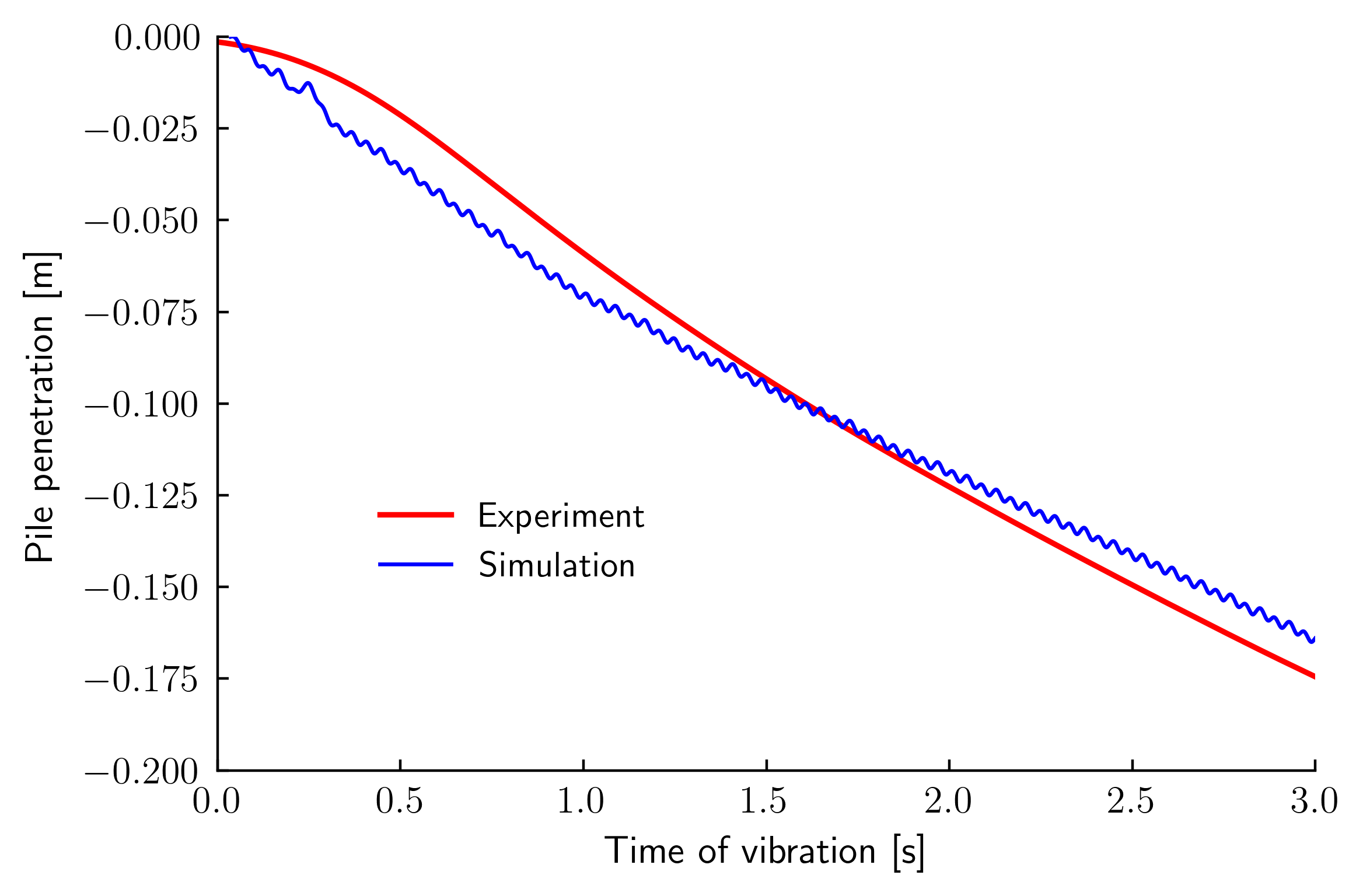 Figure 2. Pile penetration vs. time of vibration
driving
Figure 2. Pile penetration vs. time of vibration
driving
-
J. Machaček, P. Staubach, M. Tafili, H. Zachert, and T. Wichtmann. Investigation of three sophisticated constitutive soil models: From numerical formulations to element tests and the analysis of vibratory pile driving tests. Computers and Geotechnics, 138:104276, 2021. doi:10.1016/j.compgeo.2021.104276. ↩↩↩↩↩↩↩↩↩↩
-
Patrick Staubach, Jan Machaček, and Torsten Wichtmann. Mortar contact discretisation methods incorporating interface models based on Hypoplasticity and Sanisand: Application to vibratory pile driving. Computers and Geotechnics, 146:104677, jun 2022. URL: https://www.sciencedirect.com/science/article/pii/S0266352X2200043X https://linkinghub.elsevier.com/retrieve/pii/S0266352X2200043X, doi:10.1016/j.compgeo.2022.104677. ↩↩
-
C. Taylor and P. Hood. A numerical solution of the Navier-Stokes equations using the finite element technique. Computers and Fluids, 1(1):73–100, 1973. URL: https://www.sciencedirect.com/science/article/pii/0045793073900273, doi:10.1016/0045-7930(73)90027-3. ↩
-
Jakob Vogelsang, Gerhard Huber, and Theodoros Triantafyllidis. Experimental Investigation of Vibratory Pile Driving in Saturated Sand, pages 101–123. Springer International Publishing, Cham, 2017. URL: https://doi.org/10.1007/978-3-319-52590-7{\_}4, doi:10.1007/978-3-319-52590-7_4. ↩
-
Patrick Staubach, Jan Machaček, and Torsten Wichtmann. Novel approach to apply existing constitutive soil models to the modelling of interfaces. International Journal for Numerical and Analytical Methods in Geomechanics, 46(7):1241–1271, may 2022. URL: https://onlinelibrary.wiley.com/doi/10.1002/nag.3344, doi:10.1002/nag.3344. ↩
-
Jakob Vogelsang. Untersuchungen zu den Mechanismen der Pfahlrammung. PhD thesis, Veröffentlichung des Instituts für Bodenmechanik und Felsmechanik am Karlsruher Institut für Technologie (KIT), Heft 182, 2016. ↩