1D site response: Sanisand-04
Elastic first!
The current tutorial builds upon the linear elastic site response analysis presented in the previous section 1D site response: linear elastic and will only cover changes relative to the input file created there.
In the present example, we consider all four layers of the 1D soil column to be of the same material but of different relative density. For a more realistic description of soil behaviour under partially drained cyclic loading we use the Sanisand-04 constitutive model for its constitutive description.
Instead of the sinusoidal target signal used in the first example, a synthetic earthquake signal is applied to the bottom boundary of the model. The target signal is displayed in Figure 1 and be downloaded here

Figure 1. Sinusoidal target signal applied at the base of the model
The signal will be imposed using compliant base boundary conditions in order to avoid artificial reflections. Contrary to the use of Dirichlet boundary conditions (i.e. prescribing the velocities at the nodes directly) an equivalent shear force will be applied to the bottom boundary. This boundary condition is designed such that a target signal can be enforced and at the same time reflections are prevented.
Solid section
In the previous example, a homogeneous soil column was assumed (the material of layer1, layer2, layer3 and layer4 are the same). In the present study, we want to assign different material models and initial conditions to the different layers of the column.
The material behaviour of the upper most three layers will be described using the Sanisand-04 model, whereas for the material behaviour of the bottom layer linear elasticity will be used. In order to assign different material models to different parts of the model, the *Solid Section statement needs to be adapted:
*Solid Section, Elset = Soil.layer1, Material = elasto-plastic
*Solid Section, Elset = Soil.layer2, Material = elasto-plastic
*Solid Section, Elset = Soil.layer3, Material = elasto-plastic
*Solid Section, Elset = Soil.layer4, Material = elastic
The material assigned to layer1, layer2 and layer3 - Material = elasto-plastic - will be defined in the following.
Material
As already stated in the introduction, the material is considered to behave elasto-plastic in the majority of the soil column. The Sanisand-04 model is used for its constitutive description. The parameters used in this study correspond to the parameters of Nevada sand according to 1. The code snipped defining the new (elasto-plastic) material is given below:
*material, name = elasto-plastic, phases = 2

*Mechanical = Sanisand-2
100.0,0.83,0.027,0.45,1.24,0.93,0.01,103.0
0.05,18.658,1.086,1.020381,0.698,3.139,24.3,10000.0

*Optional mechanical parameter
integration, 2
tangent_stiffness, 2 ** "consistent" Jacobian
jacobi, 1            ** Elastic Jacobian
drift_correction, 0  ** If F > 0 -> adjust alpha
tol_yield, 1d-12     ** If F > 0 -> tolerance for yield surface
update_alpha, 1      ** alpha updating strategy (detect load reversal)
min_pressure, 0.5

*Density
2.2, 1.0

*Bulk modulus
1.1d6

*Permeability = isotropic
1d-12

*dynamic viscosity
1d-6

*Hourglass, stiffness = 100
Therein, the parameters are defined in the lines
*Mechanical = Sanisand-2
100.0,0.83,0.027,0.45,1.24,0.93,0.01,103.0
0.05,18.658,1.086,1.020381,0.698,3.139,24.3,10000.0
Optional mechanical parameter are used to control the numerical integration of the constitutive model. In the present example we use a Modified Euler integration scheme with automatic time stepping. In order to avoid tensile stresses, a minimum mean effective stress of \(p^\prime=0.5\) kPa (min_pressure) is enforced.
As in the linear elastic simulation, the density of the solid grains and pore water are \(\rho^s=2.2\) t/m³ and \(\rho^w=1.0\), respectively. The bulk modulus of pore water is assumed to be \(K^w=1.1\cdot 10^6\) kPa, which accounts for minor air inclusions in the ground water. The hydraulic conductivity is \(10^{-3}\) m/s and the dynamic viscosity is \(\mu^w=10^{-6}\)kPa\(\cdot\)s, resulting in a permeability of \(10^{-10}\) m².
For layer4 we choose a linear elastic constitutive model. This decision is mainly motivated by the use of a compliant base boundary condition (BC). The compliant base BC requires the definition of the impedance \(\rho c_s\) of the underlying element. In the Sanisand-04 model \(c_s\) may change significantly during the loading. In order to choose a realistic stiffness for the material and avoid unrealistic stiffness differences between layer3 (Sanisand-04) and layer4 (linear elastic), we use the elastic shear modulus of the Sanisand-04 model:
where \(G_{0}\) and \(p_{atm}\) are material parameters. Assuming a void ratio of \(e_0=0.5\) for layer3 and evaluating the mean effective stress in the middle of layer4 (\(z=75\) m) according to
with \(K_0 \approx 0.5\) leads to a shear modulus of \(G=110073\) kPa. With a Poisson's ratio of \(\nu = 0.25\) thi results in a Young's modulus of \(E=275182\) kPa. Compared to the linear elastic simulation, only the Young's modulus needs to be changed in the original material definition *Material, Name = elastic:
*Material, Name = elastic, phases = 2

*Mechanical = Linear_Elasticity
275182, 0.25
Amplitudes
The target signal is displayed in Figure 1. Such a signal could not be realized using an in-build amplitude definition of numgeo. The data of the input signal is stored in the file erdbeben-geschwindigkeit.inp, which can be downloaded here. The data is read in as an amplitude using the type = tabular option of the amplitude keyword *Amplitude:
*Amplitude, name = earthquake, type = tabular
include, input=erdbeben-geschwindigkeit
File type
Note that the file with the signal has to be of type .inp and the file ending (inp) is omitted from the command statement as shown above.
Initial conditions
The initial conditions such as void ratio (used for the calculation of porosity and densities), effective stress and pore water pressure are the same as in the linear elastic case. However, the Sanisand-04 model requires the initialisation of state variables. In the present case we initialize the void ratio used in the constitutive model to capture effects of density. State variables of constitutive models are initialized using the type = state variables sub-keyword.
Different initial void ratios are considered for the different layers:
*Initial conditions, type = state variables
soil.layer1, void_ratio, 0.65
soil.layer2, void_ratio, 0.75
soil.layer3, void_ratio, 0.55
Step 1 + 2: Geostatic and Multi-Point constraints
The boundary and loading conditions of the Geostatic and ReplaceBC steps remain unchanged. In order to have the void ratio used in the Sanisand-04 model available for output, we modify the output definition as follows:
*output, field, vtk, ASCII
...
*element output, elset = soil.all
S, E, void_ratio
Step 3: Excitation
The boundary and loading conditions of the excitation step remain unchanged, however, we changed the name of the amplitude that we want to use for load application. We further changed the elastic properties of layer4 and the impedance of the compliant base boundary condition needs to change accordingly:
*Dsload, amplitude=earthquake
bottom, compliant, 1, 419.6
With the updated elastic properties, the shear wave velocity can be calculated as \(c_s = 262\) m/s. It follows that \(\rho c_s = 419,6\) t/(ms).
As in the previous steps, the output definition is adapted to store the void ratio of the Sanisand-04 model for later inspection. We further reduce the amount of information stored during the simulation for both, the field output and the print output
*output, field, vtk, ASCII
*Frequency = 10
...
*element output, elset = soil.all
S, E, void_ratio
and
*output, print
*Frequency = 5
*node output, nset = soil.left
U, V, A
Step 4: Resting step
The last step requires similar changes as the excitation step. The impedance of the compliant base boundary condition
*Dsload, amplitude=zero
bottom, compliant, 1, 419.6
and the changes to the output definition need to be adapted:
*output, field, vtk, ASCII
*Frequency = 10
...
*element output, elset = soil.all
S, E, void_ratio
and
*output, print
*Frequency = 5
*node output, nset = soil.left
U, V, A
Results
An exemplary inspection of the simulation results is presented below. For the present example, we are interested in the question "if or if not" liquefaction occurs. A very simple way to assess potenital liquefaction is to monitor the evolution of mean effective stress
\(p^\prime\) does not exist as an output variable per default. However, Paraview offers an in-build Calculator that allows to perform mathematical operations on field variables:
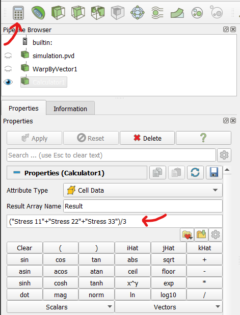
Figure 2. Calculator option of Paraview to calculate the mean effective stress
\(p^\prime = (\sigma_{11} + \sigma_{22} + \sigma_{33}) / 3\).
The distribution of the mean effective stress at different times of the dynamic simulation are depicted in Figure 3.
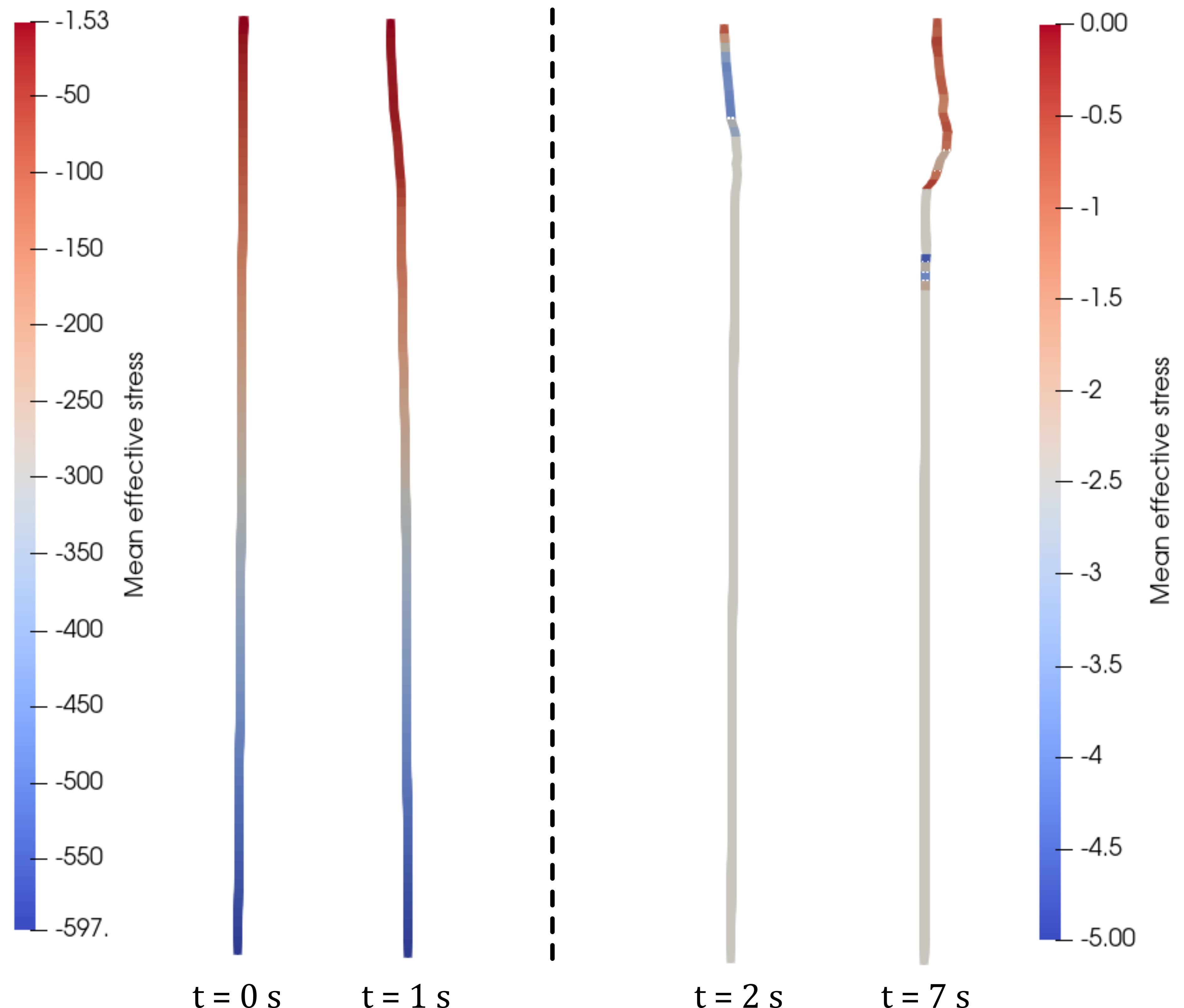
Figure 3. Distribution of mean effective stress \(p^\prime = (\sigma_{11} + \sigma_{22} + \sigma_{33}) / 3\) at different times. Deformations are shown 10 times exaggerated.
-
J. Machaček and P. Staubach, ‘Entwicklungen in der numerischen Modellierung geotechnischer Randwertprobleme’, Bautechnik, vol. 100, no. 9, pp. 1–12, 2023, doi: https://doi.org/10.1002/bate.202300060. ↩