Non-homogeneous slope (Giam & Donald 1989)
The third benchmark for strength reduction simulations features a boundary value problem presented by Giam & Donald (1989)1 as part of a survey sponsored by ACADS. The safety against failure of the non-homogeneous slope depicted in Figure 1 was evaluated using Slide2, RS2 and GeoStudio, amongst other.
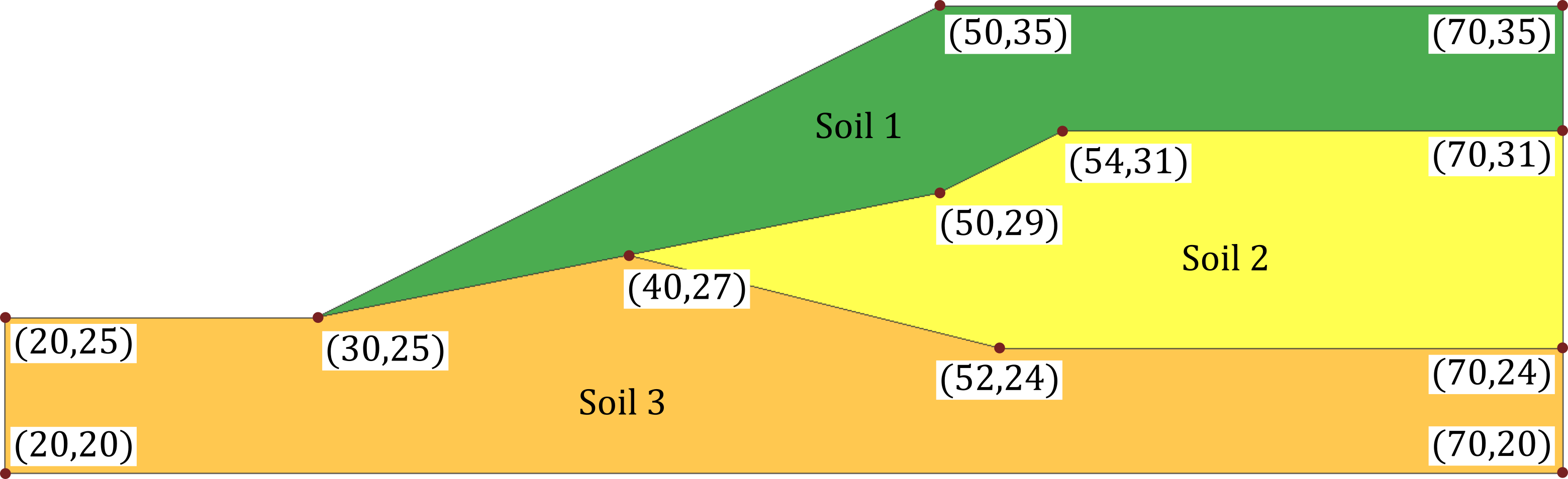
Figure 1. Geometry of the investigated slope, modified from the RS2 verification manual.
The linear elastic, perfectly plastic Mohr-Coulomb model was used in the analysis. The material properties are as follows:
Table 1. Material parameters for the strength-reduction analyses
| Soil | c (kPa) | \(\varphi\) (°) | \(\rho\) (t/m³) |
|---|---|---|---|
| 1 | 0.0 | 38 | 1.95 |
| 2 | 5.3 | 23 | 1.95 |
| 3 | 7.2 | 20 | 1.95 |
where \(c\) denotes the effective cohesion and \(\varphi\) the effective friction angle, respectively. \(\rho\) is the density of the soil. No information regarding the Young's modulus \(E\), the Poisson's ratio \(\nu\) and the dilatation angle \(\psi\) are provided. \(E=30\) MPa, \(\nu=0.3\) and \(\psi=\varphi\) are assumed. No tension cut-off is used. For the back-calculation we will use three different combinations:
- MC2: Mohr-Coulomb-2 + Default settings
- MC2-hyp: Mohr-Coulomb-2 + FoS-Hyperbolic extrapolation
- MC3: Mohr-Coulomb-3 + Default settings
Input files
The input files for the tutorial can be downloaded here. The GiD files of the finite element model are available for download as well.
Results
The resulting Factor of Safety (FoS) obtained with numgeo is compared to the results of the three different software packages (and analysis methods) in Figure 2. It can be seen that the results obtained with numgeo are within the range of results obtained with other software and are close to the once obtained with RS2.
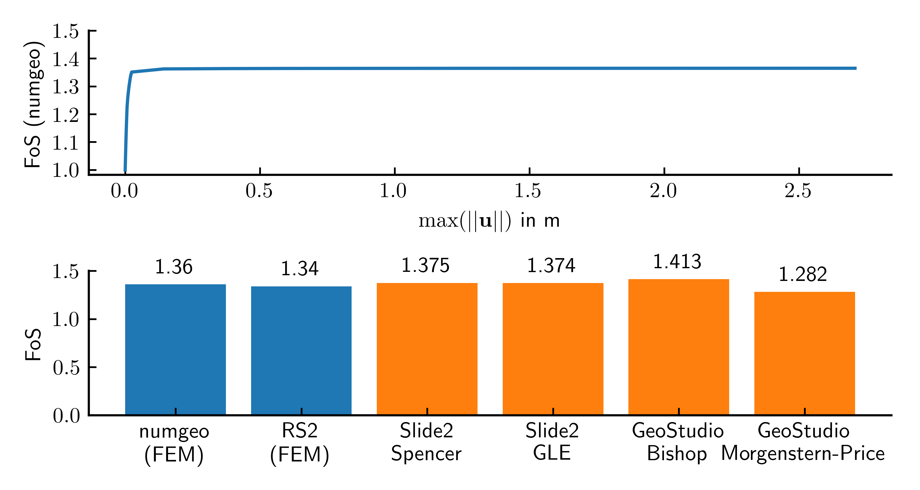
Figure 2. Max. displacement magnitude versus Factor of Safety (FoS) for case 1, calculated with numgeo (top, variant MC3) and comparison to other software (bottom).
The python script used to produce this plot is given at the end of this tutorial. The deformed geometry at failure is shown in Figure 3.
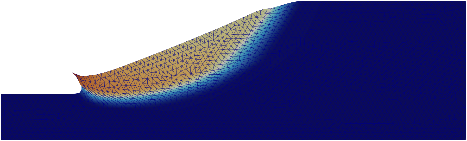
Figure 3. Deformed geometry at failure as calculated by numgeo.
#%%
import numpy as np
import matplotlib.pyplot as plt

fontsize = 9
plt.rcParams['xtick.direction'] = 'in'
plt.rcParams['ytick.direction'] = 'in'
plt.rcParams['text.usetex'] = False
plt.rcParams['font.size'] = fontsize
plt.rcParams['axes.spines.right'] = False
plt.rcParams['axes.spines.top'] = False
plt.rcParams['axes.linewidth'] = 1.0

# Convert centimeters to inches for figure sizing
def cm2inch(*tupl):
    inch = 2.54
    if isinstance(tupl[0], tuple):
        return tuple(i/inch for i in tupl[0])
    else:
        return tuple(i/inch for i in tupl)

data = np.genfromtxt('./MC2/strength-reduction-strength-reduction-history.csv', delimiter=',')
data2 = np.genfromtxt('./MC2-hyperbolic/strength-reduction-strength-reduction-history.csv', delimiter=',')
data3 = np.genfromtxt('./MC3/strength-reduction-strength-reduction-history.csv', delimiter=',')

fig, ax = plt.subplots(2,1, figsize=cm2inch(16,8), sharex=False)

ax[0].plot(data[:,1],data[:,0], ls='', marker='o', markerfacecolor=None, label='MC2')
ax[0].plot(data2[:,1],data2[:,0], ls='', marker='x', markerfacecolor=None, label='MC2 (FoS-hyperbolic)')
ax[0].plot(data3[:,1],data3[:,0], label='MC3')
ax[0].set_xlabel('$\max(||\mathbf{u}||)$ in m')
ax[0].set_ylabel('FoS (numgeo)')
ax[0].set_yticks([1., 1.1, 1.2, 1.3, 1.4])
ax[0].set_xlim(0,0.06)
ax[0].legend(frameon=False, loc='lower right')

fos = [np.round(data[-1,0],2),np.round(data2[-1,0],2),np.round(data3[-1,0],2), 1.34, 1.375, 1.374, 1.413, 1.282]
indices = np.arange(len(fos))
labels = ['numgeo \n(MC2)', 'numgeo \n(MC2-hyp)', 'numgeo \n(MC3)', 'RS2 \n(FEM)', 'Slide2 \nSpencer', 'Slide2 \nGLE', 'GeoStudio \nBishop', 'GeoStudio \nMorgenstern\n-Price']

rects = ax[1].bar(labels[0:3], fos[0:3])
ax[1].bar_label(rects, padding=3)
rects = ax[1].bar(labels[3::], fos[3::])
ax[1].bar_label(rects, padding=3)
ax[1].set_ylabel('FoS')
ax[1].set_yticks([0.0, 0.5, 1.0, 1.5])

plt.tight_layout()

plt.savefig('./acads-1-1989-results-plot.png', dpi=600)
-
I.B. Donald, P.S.K. Giam, and Monash University. Department of Civil Engineering. Example Problems for Testing Soil Slope Stability Programs. Civil engineering research reports Monash University. Department of Civil Engineering, Monash University, 1989. ISBN 9780867469219. URL: https://books.google.de/books?id=TfOqYgEACAAJ. ↩