Shallow unconfined flow with rainfall

The problem considered in this section involves the infiltration of water downward through soil. It is characterized by a boundary of flow domain also known as a free surface. Such a problem domain is said to be unconfined. Water may infiltrate downward through the soil due to rainfall or artificial infiltration. Rainfall is presented as a uniform discharge Q of \(2.5 \cdot 10^{-6}\) m/s, defined as the amount of water per unit area that enters the aquifer per unit time. Figure 1 shows the problem of flow between two long and straight parallel rivers, separated by a section of land. The free surface of the land is subjected to rainfall

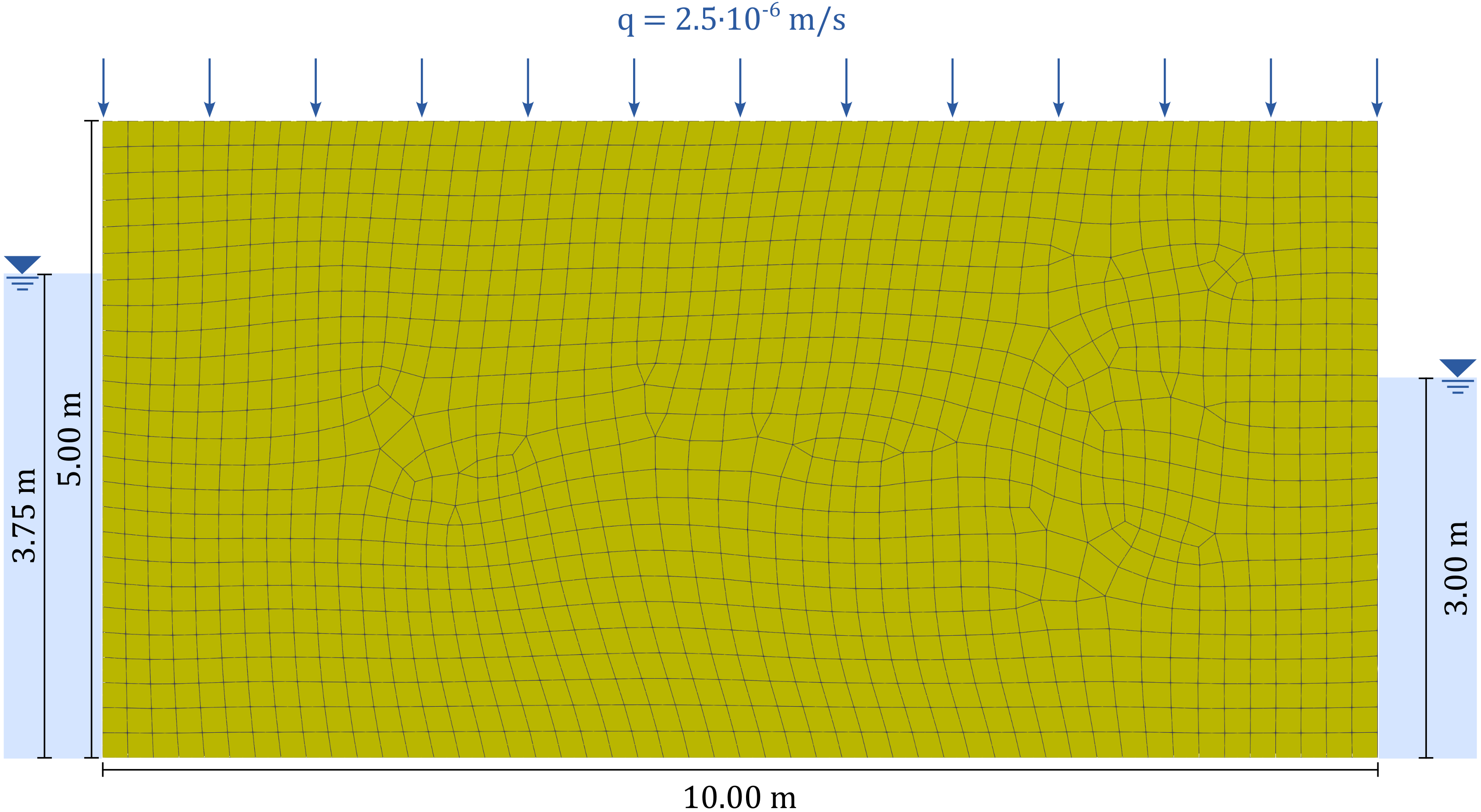
Figure 1. Problem setting and representative finite element mesh of the shallow unconfined flow with rainfall boundary value problem.

For the solid a linear elastic constitutive model is chosen. As no soil deformation is considered in this simulation (an neither was observed in the experiment) this choice is completely arbitrary. The Young's modulus is \(30 \cdot 10^3\) kPa and the Poisson's ratio \(0.3\). The hydraulic conductivity of the soil is \(10^{-5}\) m/s. Note that numgeo requires the prescription of the permeability \(K^s\) of the solid and the dynamic viscosity of the pore fluids \(\mu^f\) instead of the hydraulic conductivity \(K^f= \dfrac{K^s \gamma^f}{\mu^f}\). \(\gamma^f\) and \(\mu^f\) are the specific weight and the dynamic viscosity of the fluid \(f\), respectively.

The dynamic viscosity of pore water is \(\mu^w=10^{-6}\) kPa\(\cdot\)s and of the pore air \(\mu^a=10^{-8}\) kPa\(\cdot\)s. Assuming a specific weight of 10 kN/m³ for the pore water, the permeability of the soil is calculated to \(1 \cdot 10^{-12}\) m².

For unsaturated flow simulations numgeo requires information on the soil-water retention curve (hydraulic model) and the relative permeability model. For the present example, the well van Genuchten model was used with the model constants \(\alpha_{vG}=0.06\) and \(n_{vG}=3\). The constants were chosen arbitrarily and represent a marl. Note that the choice of SWRC (and model constants) influences the location of the phreatic surface.

The model was discretised using "flow-only" p8 and p6 elements with an average mesh size of 0.2 m, resulting in a total of 1273 elements and 3956 nodes.

Input files

The input files for the benchmark simulation can be downloaded here

Analytical solution

The analytical (steady-state) solution for this problem is presented e.g. in Harr (1991)¹. The maximum elevation of the free surface can be calculated as

\[ x_{max} = \dfrac{L}{2} \left( 1 - \dfrac{K^f}{Q} \dfrac{h_1^2-h_s^2}{L^2} \right) \]

where \(L\) is the width of the land section of the model and \(h_1\) and \(h_2\) are the water table heights on the left and the right side of the model, respectively. The corresponding maximum height for the free surface is

\[ h_{max} = \sqrt{ h_1^2 - \dfrac{x_{max}}{L}\left(h_1^2-h_s^2\right) + \dfrac{}{} \left(L-x_{max}\right)x_{max} } \]

Results

The pore water pressure distribution and location of the phreatic surface calculated with numgeo are depicted in Figure 2. The maximum elevation of the phreatic surface is \(h_{max}^{FEM}=4.55\) m at a location of \(x_{max}^{FEM}=4.03\) m.

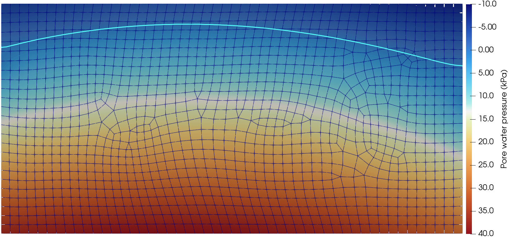
Figure 2. Simulation results: Pore water pressure contour plot and location of phreatic surface (cyan).

The same problem was studied by rocscience for the verification of the finite element software RS2 and RS3. A comparison of the simulation results obtained with numgeo and reported by rocscience with the analytical solution is provided in the following table.

	Analytical	numgeo	RS2	RS3
\(x_{max}\) (m)	3.99	4.03	4.22	4.25
\(h_{max}\) (m)	4.25	4.55	4.52	4.46

As already noted in the introduction, the exact value of \(h_{max}\) - evaluated as the maximum elevation fo the phreatic surface, i.e. the surface for which the condition \(p^w=0\) kPa holds - depends on the SWRC. The SWRC is not considered in the analytical solution and no information is provided for RS2 and RS3 in this regard. Some deviations are thus to be expected. Overall, the results are in close agreement.

Automatic Benchmark results

This benchmark is part of an automated test suite executed before every software release to ensure the accuracy and reliability of the code. The following table shows the performance of the current numgeo release by comparing its results against a known analytical solution.

Automating the evaluation of the phreatic line and performing a maximum search on it is rather complicated. Therefore, for the automatic benchmark, the pore water pressure at two discrete points, the top left and top right corners of the model, are compared. As a reference, the results of the finite element simulation shown in Figure 2 are used as they match well the analytical and the rocscience results.

A comparison of the different element types available in numgeo and their performance in this benchmark is given below.

	p8	p6	u8p8-stab	u6p6-stab	u8p4	u6p3
\(\Delta p^w_{left}\) (%)	0	-0.068	2.785	2.754	-1.307	-2.4
\(\Delta p^w_{right}\) (%)	0	-0.001	2.73	2.77	-1.314	-2.585

Milton Edward Harr. Groundwater and Seepage. Courier Corporation, 1991. ↩