Cone Penetration Test (CPT) Benchmark: Mohr-Coulomb, Updated Lagrange (numgeo vs Abaqus)

This benchmark presents a cone penetration test (CPT) simulation comparing numgeo and Abaqus. Both finite element models use identical boundary conditions, contact definitions, material behavior, mesh topology, and loading characteristics. The purpose is to validate consistency in cone resistance predictions. The CPT is modeled as an axisymmetric, dynamic penetration of a rigid cone into dry sand. The simulation is performed using a constant penetration rate.

Horizontal stress distributions during cone penetration using Abaqus and numgeo are depicted in Figure 1. It is visible that this benchmark also considers large deformations of the soil, which are performed in an Updated Lagrangian scheme. The benchmark also serves to validate the contact implementations in numgeo as well as the definition of the friction between the cone and the soil.

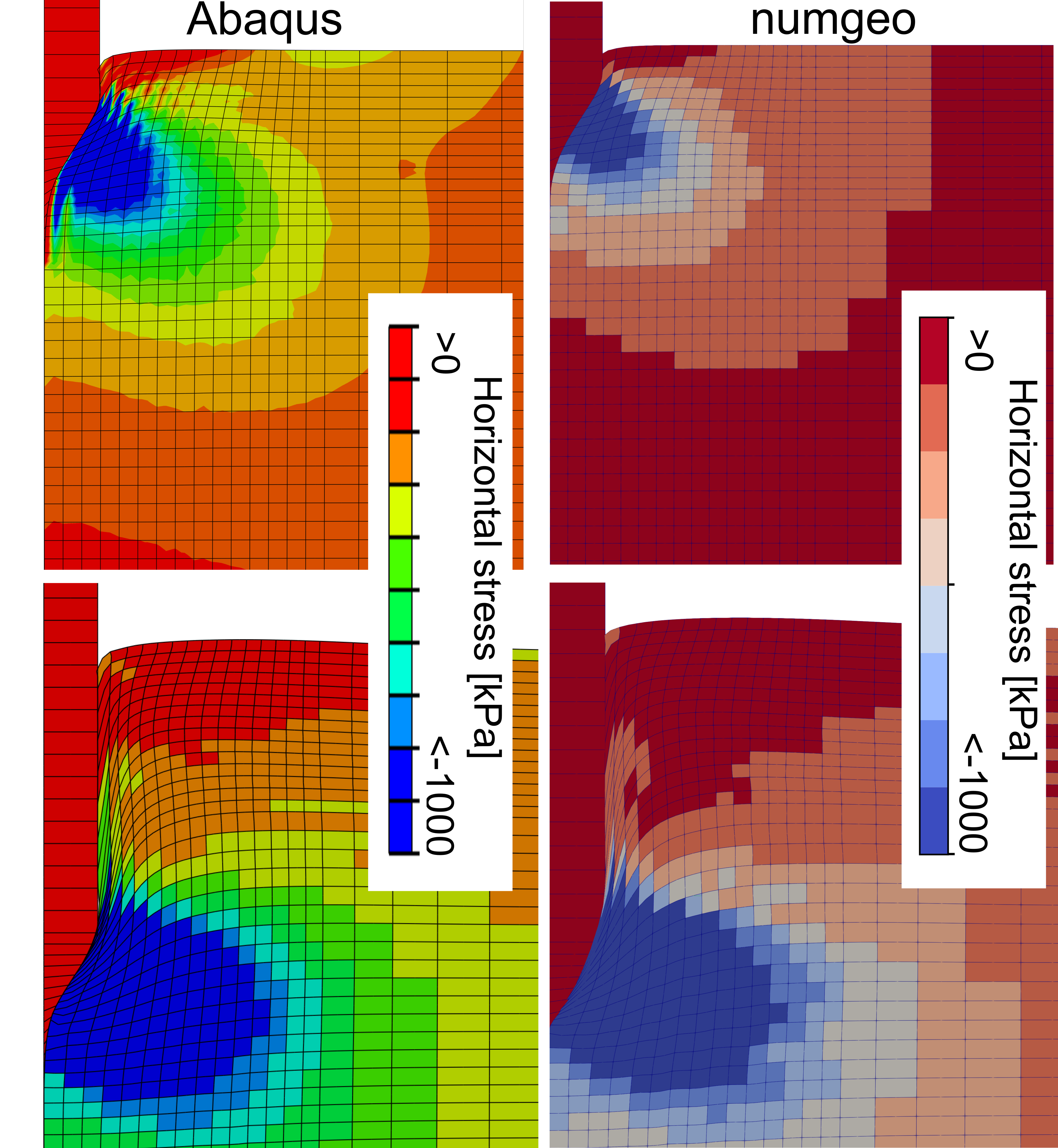
Figure 1. Horizontal stress distributions during cone penetration using Abaqus and numgeo

Tip

The input files for 2D benchmark simulations can be downloaded here.

Material Model

In numgeo, the soil is modeled using the built-in Mohr–Coulomb model. The material definition includes:

*Material, name=soil, phases=1
*Mechanical = Mohr-Coulomb-2
50d3, 0.3, 5, 0.52, 0.17, 0.
*Density
1.42d0

The Mohr–Coulomb keyword expects:

• Young’s modulus \(E = 30000\) kPa
• Poisson’s ratio \(\nu = 0.3\)
• Cohesion \(c = 5.0\) kPa
• Friction angle \(\phi = 0.52\) rad
• Dilation angle \(\psi = 0.17\) rad
• Tension cut value \(p_t = 0\) kPa

In Abaqus, no user subroutines are employed. All modeling features are implemented using built-in capabilities, including the Mohr–Coulomb model:

*Elastic
50d3, 0.3
*MOHR COULOMB
29.8,9.74
*MOHR COULOMB HARDENING
5,0
5,0.1
*Density
1.42

Boundary Conditions and Loading Definition

Penetration is enforced by prescribing a vertical displacement of the cone tip via a ramp amplitude:

*AMPLITUDE, NAME = LoadingRamp20mms , TYPE = RAMP
0.0, 0.0, 20.0, 1.00

A surface load is applied to the top boundary of the soil domain to simulate overburden stress:

*Dsload,instant
surf_soil_top, P, -107

The lateral displacements of the entire cone are fixed to zero in the horizontal direction, the bottom of the soil is restrained in vertical direction, and the right boundary is prevented from moving horizontally.

*BOUNDARY
cpt_all, u1, 0.0d0
soil_bottom,u2, 0.0d0
soil_right, u1, 0.0d0

*Boundary, amplitude=LoadingRamp20mms
cpt_top_left, u2, -1.0

This setup simulates a constant-rate penetration using the pre-defined amplitude.

Contact and Interface Conditions

Both models define frictional contact with possible separation of the surfaces. This means normal contact is enforced with allowing detachment, while frictional slip is controlled by a Coulomb law.

In numgeo, this is defined using:

*INTERACTION, name = penalty, MECHANICAL = penalty, stiffness_factor=40, user
*friction, model = MC
*Contact Pair, interaction = penalty, discretisation = element mortar
surf_soil_CPT, surf_CPT_soil

• stiffness_factor assigns a two times higher penalty value than the default setting. In the results section at the end of this page simulation results using the default value are discussed as well.
• user indicates the usage of user_contact_properties to define friction

To define friction, a user subroutine user_contact_properties is used in numgeo. This allows:

• Definition of the tangential stiffness \(\varepsilon_T\) of the Coulomb contact law, see also the theory manual
• Selective activation of the friction coefficient only on the CPT shaft and sides, not at the extended tip (Zipper method)

The subroutine logic:

• Sets props(1) = \(\varepsilon_T\)
• Activates friction props(2) = \(\mu = 0.381\) only when the contact point lies at the shaft or tip and not at the zipper extension
• Friction is deactivated at the extended tip, necessary for the Zipper-based penetration

props(:) = 0.0d0
props(1) = 30d4  ! Tangential stiffness
if (y >= yref1 .and. y <= yref2) then
  props(2) = 0.381  ! Friction coefficient
endif

This refinement is not possible via keyword input alone.

Three different simulations with varied \(\varepsilon_T\) values are compared to assess the sensitivity of cone resistance to tangential contact stiffness.

In Abaqus:

*Surface Interaction, name=IntProp-1
1.,
*Friction, dependencies=1
 0.0, , ,0 ,0,0
0.381, , ,0.5 ,0.5,0.5
*Contact, op=NEW
*Contact Inclusions, ALL EXTERIOR
*Contact Property Assignment
 ,  , IntProp-1

In Abaqus, achieving a spatially selective assignment of friction can be realized by using field variables that distinguish between the CPT shaft and tip (where friction is applied) and the extended lower part of the cone (where friction must be deactivated due to the Zipper method):

*INITIAL CONDITIONS,TYPE=FIELD 
cpt_tip,1
cpt_shaft,1
soil_all,0

Comparison of Results

The following figures summarize the simulation results with varying tangential stiffness \(\varepsilon_T\) in numgeo and simulations using Abaqus. Both simulations produce a force–time curve showing cone resistance. The results are post-processed in Python using the script provided here.

It is visible that with decreasing tangential stiffness factor, the oscillations in the numerical results of numgeo get less. This is typically what is to be expected because the higher the tangential stiffness factor, the more rigorously the sticking and sliding behavior of the Coulomb friction model will be enforced. Similarly, Abaqus uses the slip tolerance with a fixed value and also shows higher oscillations if the slip tolerance decreases (not shown here).

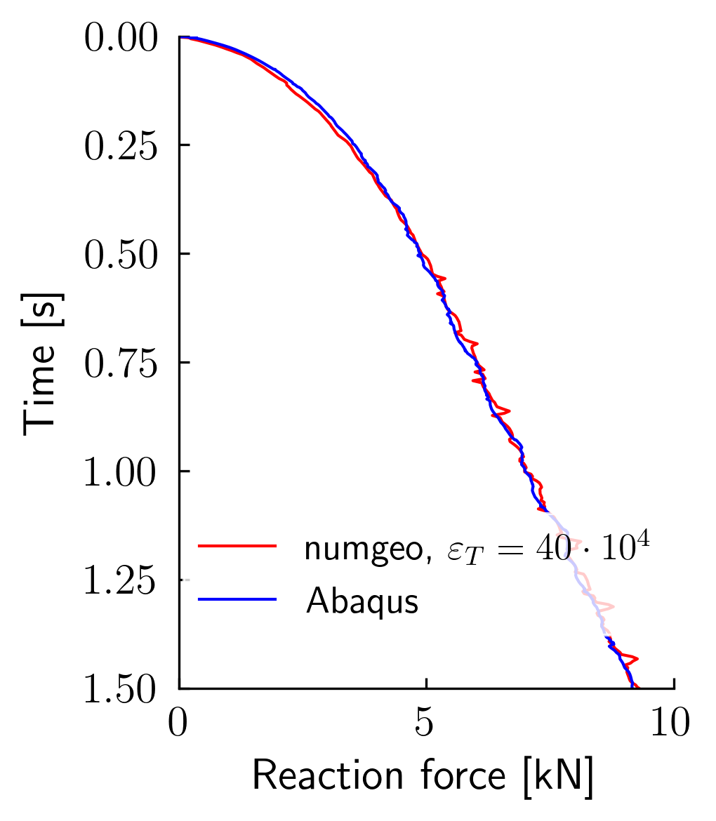
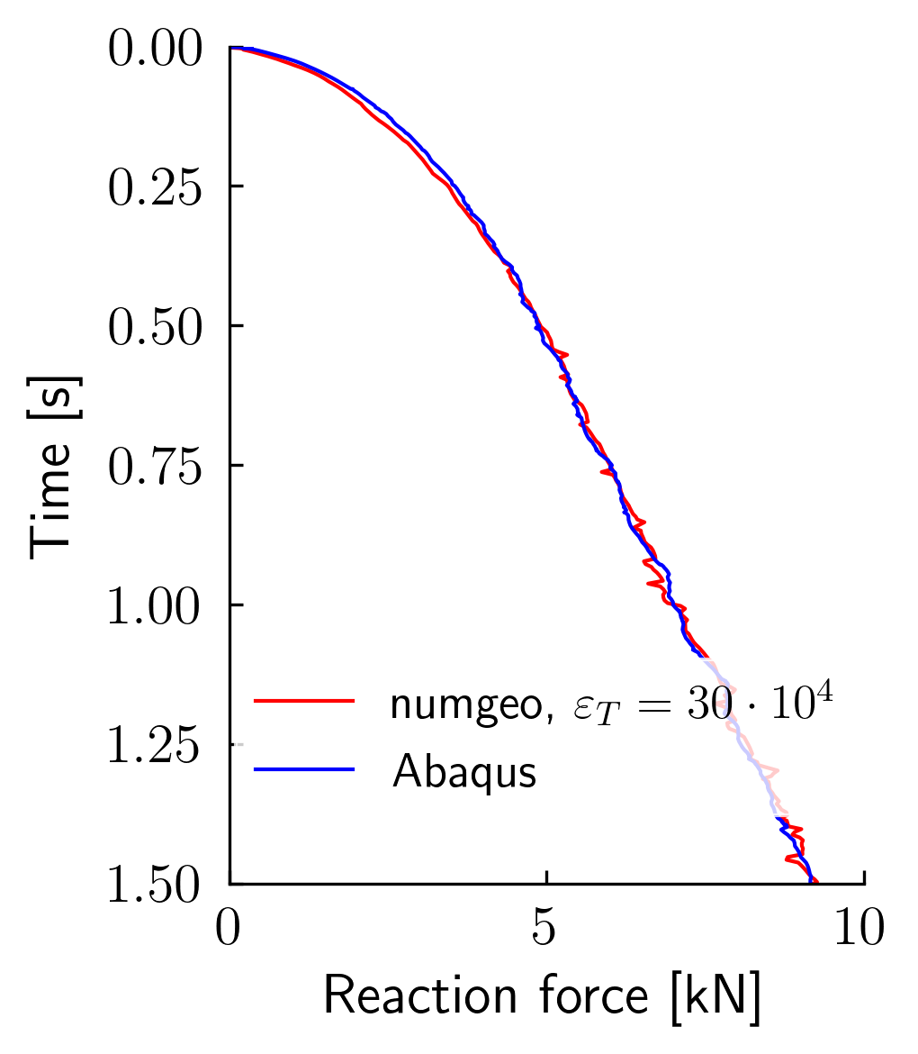
Figure 2. Comparison of three CPT simulations with varying tangential stiffness in numgeo with simulations using Abaqus.

As discussed earlier, the stiffness_factor is assigned a value two times than the default setting. Therefore, the penalty factor is defined as forty times the underlying material stiffness of the soil. Figure 3 shows the results for the default value of twenty times the underlying material stiffness of the soil. The oscillation in the results cleary increases. This is specifically a problem of the CPT simulations because the normal contact stiffness is evaluated bases on the initial soil stiffness. However, when the CPT penetrates into the soil, stresses increase sharply, leading to an increase in stiffness. Since this is not accounted for in the normal contact stiffness, the soil tends to overlap with the CPT tip, leading to oscillations in the results.

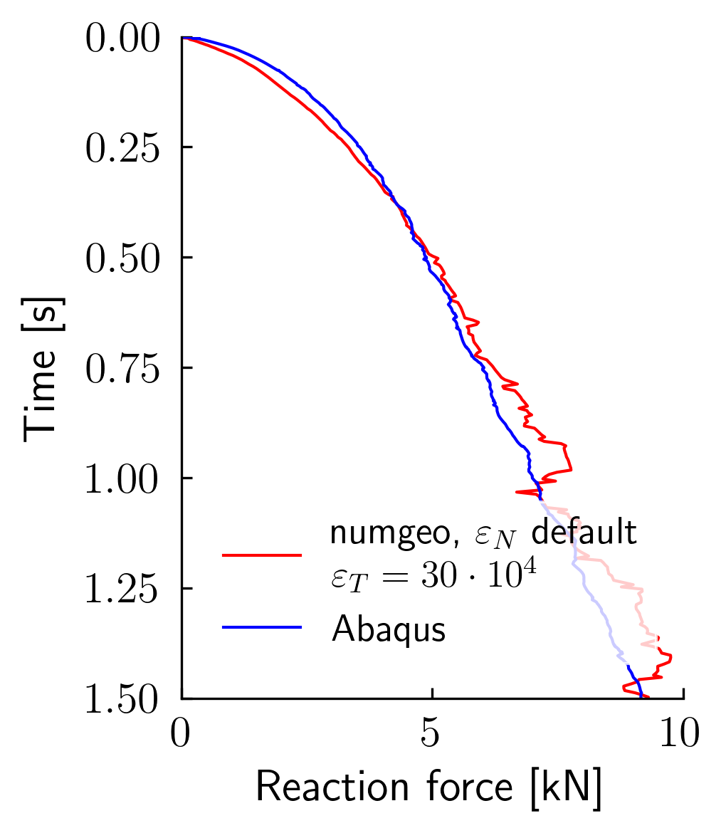
Figure 3. Comparison of the CPT simulations with the default normal contact stiffness in numgeo with simulations using Abaqus.