Triaxial Test - Consolidated Drained Cyclic Loading using the HCA Model

Finite Element (FE) representation

For the simulation of consolidated drained (CD) cyclic triaxial test using the HCA model we perform a so-called ''single-element-simulation'' and by doing so enforce element test assumptions, i.e. a homogeneous distribution of stress/strain within the test sample. A schematic of the FE representation of the CD test is given below.

triaxCD

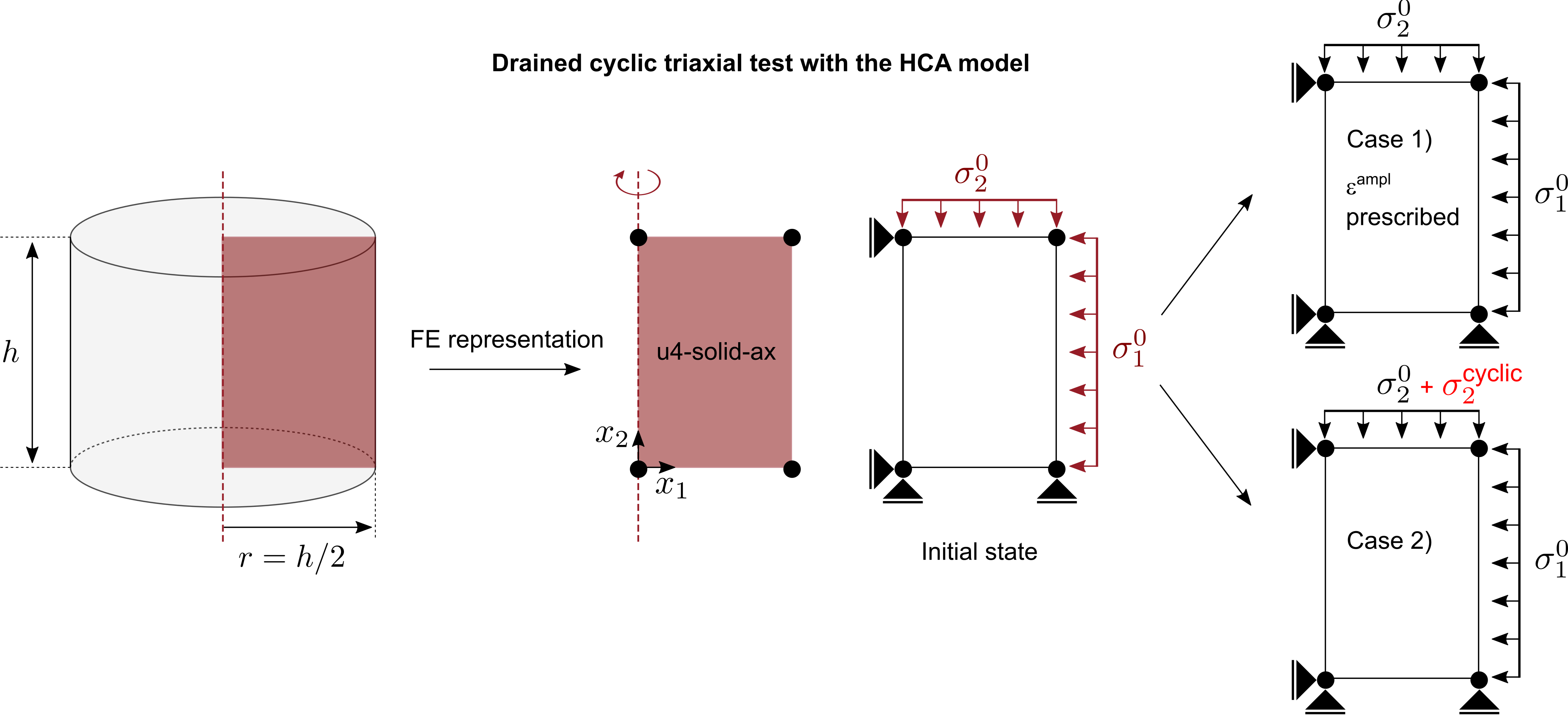
In a first initial step, the initial conditions are applied, i.e. initial stress (\(\sigma_1^0, \sigma_2^0\)), initial void ratio \(e_0\) or any other initial state variable required by the constitutive model.

Two different cases are then simulated:

Case 1): The strain amplitude \(\varepsilon^{ampl}\) is prescribed as initial condition without explicitly calculating it. In the second HCA step, the accumulation of deformations due to \(10^6\) cycles are simulated using the HCA model with a given strain amplitude of \(\varepsilon^{ampl}=8 \cdot 10^{-4}\).
Case 2): The strain amplitude is calculated by simulating an individual cycle and recording the strain path. The hypoplastic model with intergranular strain extension is used to simulate two individual cycles (of which the second is used to calculate the strain amplitude). The HCA phase follows in the fourth step.

Constitutive model

The HCA model is used in combination with the hypoplastic model with intergranular strain extension for this example. The parameters for "Karlsruhe fine sand" for the HCA model are used and provided in the Table below.

\(C_{\textrm{ampl}}\)	\(C_{e}\)	\(C_{p}\)	\(C_{Y}\)	\(C_{N1}\)	\(C_{N2}\)	\(C_{N3}\)
1.33	0.60	0.23	1.68	2.95\(\cdot10^{-4}\)	0.41	\(1.9 \cdot 10^{-5}\)

Model generation

As single-element simulations do not involve complex geometries, we do not use a pre-processor and generate the input file by hand.

First we create the four nodes defining the finite element:

*Node
1, 0.0 , 0.00
2, 0.05, 0.00
3, 0.05, 0.1
4, 0.00, 0.10

We use an axisymmetric four node solid element (only one phase considered)
```
*Element, type = U4-solid-ax-red
1, 1, 2, 3, 4
```

Next, we define some node and element sets for the assignment of boundary conditions, loads and material parameters:

*Nset, Nset = nall
1, 2, 3, 4
*Nset, Nset = nleft
1, 4
*Nset, Nset = nright
2 , 3
*Nset, Nset = nbottom
1 , 2
*Nset, Nset = ntop
3 , 4
*Elset, Elset=eall
1

In order to assign the material to the element, we first create a solid section. The material name linked to this solid section is arbitrary but must be specified in a later step.
```
*Solid Section, elset = eall, material = soil
```

Sample numgeo input file using the strain amplitude from the experiment as input

In the first example, the strain amplitude is not calculated by a conventional constitutive model, but a measured amplitude from an experiment is used. This is typically the case if the simulations are performed to calibrate or check the parameters of the HCA model.

Define the material: In addition to the material parameters, the HCA model requires the declaration of the step types. The first step is a low-cycle ("implicit") step. The actual HCA phase is performed in step HCA. The period of the cycles is 1.

*Material, name = soil, phases = 1

*Mechanical = HCA_Linear_Elasticity
5000.0,0.32
** Parameters of Karlsruhe fine sand
**CN1, CN2, CN3, Campl, Ce, 0, Cp2, 0
**Cy2, Cpi1, Cpi2, Cpi3, patm, eref, eps^ampl_ref, A
**a, n, nu, phic
0.000295,0.41,1.9e-05,1.33,0.6,0,0.23,0,
1.68,0,0,0,100.0,1.054,0.0001,1209,
1.63,0.5,0.32,0.578

*Density
2.65

*Implicit hca steps
Geostatic
*Explicit hca steps
HCA
*HCA cycle time
1

Define the initial conditions of the simulation. In the present case this comprises the definition of the initial (effective) stresses, the initial void ratio and the strain amplitude. A value of \(\varepsilon^{ampl}=8 \cdot 10^{-4}\) is set.
```
*Initial conditions, type=stress, geostatic
eall, 0.0, -150.0,  0.10, -150.0, 1.0, 1.0

*Initial conditions, Type = state variables
** Initial relative density of 80 %
eall, void_ratio, 0.818
eall, strain_ampl, 8d-4
```
As in most simulations in geotechnical engineering we start the simulation by initializing the geostatic stress field due to the self weight of the soil and any initial external loading without generating any deformations. In the present case, the initial stress field is solely given by the external load of 150 kPa acting isotropically on the sample. Since this is a very basic simulation, we do not request a field output but rely solely on the print output for evaluating the simulation results.
```
*Step, name = Geostatic
*Geostatic

*Body force, instant
eall, grav, 10.0, 0., -1, 0.
*Dload, instant
eall, p3, -150
*Dload, instant
eall, p2, -150
*Boundary
nleft, u1, 0.
nbottom, u2, 0.

*End Step
```
In the second step, \(10^6\) cycles are simulated using the HCA model. The initial increment is 0.2, the total step time is \(10^6\), the minimum allowed increment is 0.0001 and the maximum increment is \(10^4\). Note that time does not correspond to physical time in a static step but corresponds in the present case to the number of cycles being simulated. The static analysis type indicates that no inertia forces (and therefore no physical time dependencies) are considered. During the analyses, the average stresses are kept constant. The soil sample is free to settle and deform radially.
```
** ----------------------------------------

*Step, name = HCA, inc = 10000000
*Static
0.2, 1d6, 0.0001,1d4

*Body force, instant
eall, grav, 10.0, 0., -1, 0.
*Dload, instant
eall, p3, -150
*Dload, instant
eall, p2, -150
*Boundary
nleft, u1, 0.
nbottom, u2, 0.

*output,print
*Element output, Elset = eall
S, E, void_ratio, strain_ampl
*End Step
```
We end the input file by using the "End Step" command.
```
*End Input
```

Results

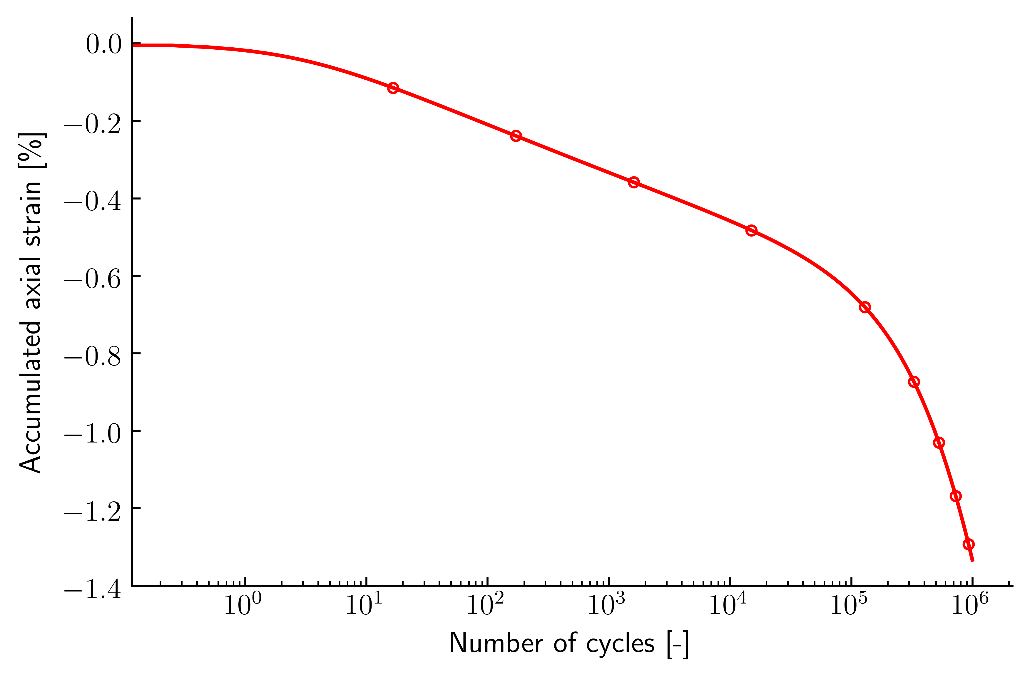
The accumulated permanent axial strain versus number of load cycles is given in Figure 2.

triaxCDHCAinput

Python Script for plotting the results

The python script used to generate Figure 2 is given below:

import matplotlib
import matplotlib.pyplot as plt
import matplotlib.ticker as mtick
from pylab import genfromtxt
from matplotlib import rc
import os 
import numpy as np
dir_path = os.path.dirname(os.path.realpath(__file__))
plt.rcParams['backend'] = "pdf"
plt.rcParams['xtick.direction'] = 'in'
plt.rcParams['ytick.direction'] = 'in'
plt.rcParams['text.usetex'] = True
plt.rcParams['font.size'] = 12
plt.rcParams['axes.spines.right'] = False
plt.rcParams['axes.spines.top'] = False
plt.rcParams['axes.linewidth'] = 0.8 


#=============================================================================
# Read data
#%% =============================================================================


dirname = '/step-print-out'

dir_path = os.path.normpath(os.getcwd() +dirname)

sim1 = genfromtxt(dir_path+'/'+'EALL_element_1.dat',skip_header=2)

#=============================================================================
# Plot first data
#%% =============================================================================
plt.figure(1)
plt.subplot(111)

plt.semilogx(sim1[:,0]-sim1[0,0],sim1[:,7]*100,'or-', \
         markersize=4,markerfacecolor='none',markevery=20,\
         label=r'Simulation',clip_on=True)

ax = plt.gca()
ax.set_xlabel(r'Number of  cycles [-]')
ax.set_ylabel(r'Accumulated axial strain [\%]',labelpad=7)

plt.tight_layout() 
fig = plt.gcf()  
fig.savefig('accumulated_permanent_strain_drained_input_epsampl.pdf', dpi=600 , bbox_inches='tight')
fig.savefig('accumulated_permanent_strain_drained_input_epsampl.png', dpi=600 , bbox_inches='tight')

Sample numgeo input file calculating the strain amplitude with a conventional model

In the second example, the strain amplitude is calculated by a conventional constitutive model, the hypoplastic model with intergranular strain extension in the present case. Having to calculate the strain amplitude is the case for a typical boundary value problem.

Only the required modifications of the first example are explained in the following. The rest of the input file remains identical.

The first two steps are low-cycle ("implicit") steps. The sinusoidal load is applied in FirstCycle and in SecCycle, whereby the strain curve is recorded for the latter. The actual HCA phase is performed in the step named HCA. The period of the cycles is 1.

*Material, name = soil, phases = 1

** Parameters of Karlsruhe fine sand
*mechanical = HCA_Hypoplasticity
**phi, nu, hS, n, ed0, ec0, ei0, alpha
**beta, mT, mR, R, betaR, chi, Kw
0.577, 0.0, 4d6, 0.27, 0.677, 1.054, 1.15, 0.14
2.5, 1.2, 2.4, 1d-4, 0.1, 6.0 , 0.
*******
**CN1, CN2, CN3, Campl, Ce, 0, Cp2, 0
**Cy2, Cpi1, Cpi2, Cpi3, patm, eref, eps^ampl_ref, A
**a, n, nu, phic
0.000295, 0.41, 0.000019, 1.33, 0.6, 0, 0.23, 0
1.68, 0, 0, 0, 100, 1.054, 0.0001, 1209
1.63, 0.5, 0.32, 0.577

*Density
2.65

*Implicit hca steps
Geostatic, FirstCycle
*Recording hca steps
SecCycle
*Explicit hca steps
HCA
*HCA cycle time
1

To apply cyclic loading, a sinusoidal amplitude with a frequency of 1 Hz is defined in addition.
```
*Amplitude, name = sine1Hz, Type=periodic
1, 0.0, 0.0, 6.283
0.0, 1.0
```

In the second and third step, one individual cycle is simulated in each step. The steps are defined identical.

*Step, name = FirstCycle, inc = 10000000
*Static
0.02, 1, 0.0001, 0.02

*Body force, instant
eall, grav, 10.0, 0., -1, 0.
*Dload, instant
eall, p3, -150
*Dload, instant
eall, p2, -150

*Dload, amplitude=sine1Hz
eall, P3, -60

*Boundary
nleft, u1, 0.
nbottom, u2, 0.

*output,print
*Element output, Elset = eall
S, E, void_ratio, strain_ampl
*End Step

** ----------------------------------------

*Step, name = SecCycle, inc = 10000000
*Static
0.02, 1, 0.0001, 0.02

*Body force, instant
eall, grav, 10.0, 0., -1, 0.
*Dload, instant
eall, p3, -150
*Dload, instant
eall, p2, -150

*Dload, amplitude=sine1Hz
eall, P3, -60

*Boundary
nleft, u1, 0.
nbottom, u2, 0.

*output,print
*Element output, Elset = eall
S, E, void_ratio, strain_ampl
*End Step

The HCA step remains unchanged.

Results

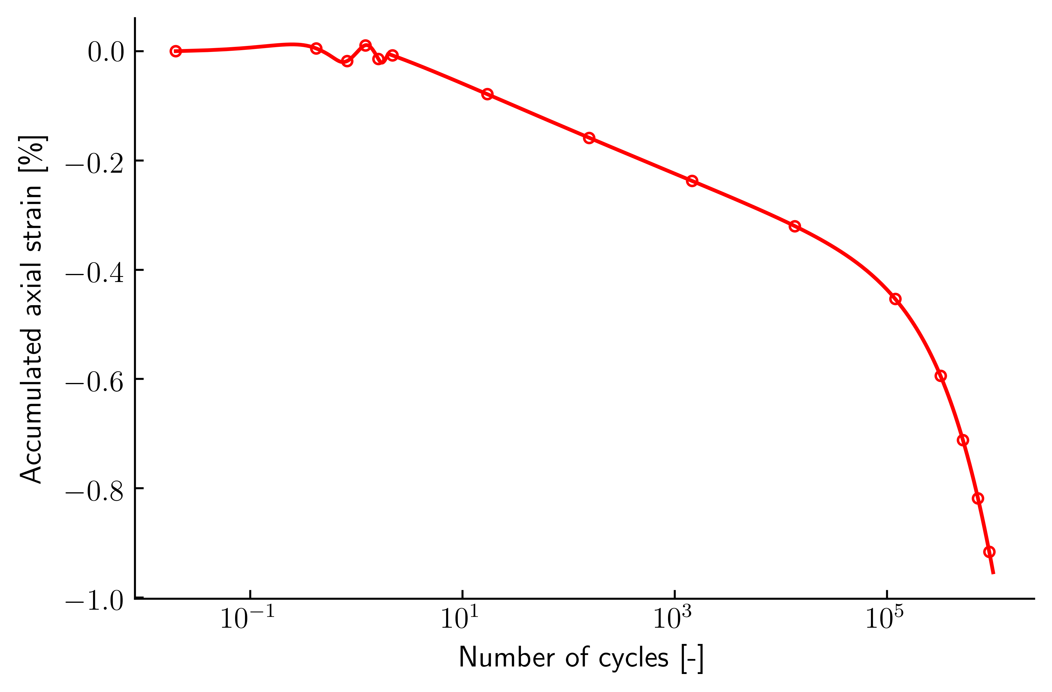
The accumulated permanent axial strain versus number of load cycles is given in Figure 3. The simulated individual cycles are well visible. The strain amplitude calculated using the hypoplastic model with intergranular strain extension is approximately \(\varepsilon^{ampl}=5.6 \cdot 10^{-4}\) (see the print output), which is slightly lower than in the first example and results in less accumulated strain during the HCA phase.

triaxCDHCAcalculated

Complete input file for a predefined strain amplitude

The complete input file is given below.

**=~~=~~=~~=~~=~~=~~=~~=~~=~~=~~=~~=~~=~~=~~=~~=~~=~~=~~=~~=~~=~~=~~=~~=~~=~~=
**                                  numgeo                                    
**             Copyright (C) 2024 Jan Machacek, Patrick Staubach              
**=~~=~~=~~=~~=~~=~~=~~=~~=~~=~~=~~=~~=~~=~~=~~=~~=~~=~~=~~=~~=~~=~~=~~=~~=~~=

**=~~=~~=~~=~~=~~=~~=~~=~~=~~=~~=~~=~~=~~=~~=~~=~~=~~=~~=~~=~~=~~=~~=~~=~~=~~=
**
**
** For this simple problem we do not need to define any parts or sections
**
**
*Node
1, 0.0 , 0.00
2, 0.05, 0.00
3, 0.05, 0.1
4, 0.00, 0.10

*Nset, Nset=nall
1, 2, 3, 4, 5
*Nset, Nset=nleft
1, 4
*Nset, Nset=nright
2 , 3
*Nset, Nset=nbottom
1 , 2
*Nset, Nset=ntop
3 , 4

*Element, type = U4-solid-ax-red
1, 1, 2, 3, 4

*Elset, Elset=eall
1

** ----------------------------------------

*Solid Section, Elset = eall, material=soil

** ----------------------------------------

*Material, name = soil, phases = 1

*Mechanical = HCA_Linear_Elasticity
5000.0,0.32
** Parameters of Karlsruhe fine sand
0.000295,0.41,1.9e-05,1.33,0.6,0,0.23,0,
1.68,0,0,0,100.0,1.054,0.0001,1209,
1.63,0.5,0.32,0.578

*Density
2.65


*Implicit hca steps
Geostatic
*Explicit hca steps
HCA
*HCA cycle time
1

** ----------------------------------------

*Initial conditions, type=stress, geostatic
eall, 0.0, -150.0,  0.10, -150.0, 1.0, 1.0

*Initial conditions, Type = state variables
** Initial relative density of 80 %
eall, void_ratio, 0.818
eall, strain_ampl, 8d-4

** ----------------------------------------

** ----------------------------------------

*Step, name = Geostatic
*Geostatic

*Body force, instant
eall, grav, 10.0, 0., -1, 0.
*Dload, instant
eall, p3, -150
*Dload, instant
eall, p2, -150
*Boundary
nleft, u1, 0.
nbottom, u2, 0.

*End Step

** ----------------------------------------

*Step, name = HCA, inc = 10000000
*Static
0.2, 1d6, 0.0001,1d4

*Body force, instant
eall, grav, 10.0, 0., -1, 0.
*Dload, instant
eall, p3, -150
*Dload, instant
eall, p2, -150
*Boundary
nleft, u1, 0.
nbottom, u2, 0.

*output,print
*Element output, Elset = eall
S, E, void_ratio, strain_ampl, strain_acc, cyclic_history, fampl, fe, fp, fY
*End Step

** ----------------------------------------

*End Input

Complete input file calculating the strain amplitude

The complete input file is given below.

**=~~=~~=~~=~~=~~=~~=~~=~~=~~=~~=~~=~~=~~=~~=~~=~~=~~=~~=~~=~~=~~=~~=~~=~~=~~=
**                                  numgeo                                    
**             Copyright (C) 2024 Jan Machacek, Patrick Staubach              
**=~~=~~=~~=~~=~~=~~=~~=~~=~~=~~=~~=~~=~~=~~=~~=~~=~~=~~=~~=~~=~~=~~=~~=~~=~~=

**=~~=~~=~~=~~=~~=~~=~~=~~=~~=~~=~~=~~=~~=~~=~~=~~=~~=~~=~~=~~=~~=~~=~~=~~=~~=
**
**
** For this simple problem we do not need to define any parts or sections
**
**
*Node
1, 0.0 , 0.00
2, 0.05, 0.00
3, 0.05, 0.1
4, 0.00, 0.10

*Nset, Nset=nall
1, 2, 3, 4
*Nset, Nset=nleft
1, 4
*Nset, Nset=nright
2 , 3
*Nset, Nset=nbottom
1 , 2
*Nset, Nset=ntop
3 , 4

*Element, type = U4-solid-ax-red
1, 1, 2, 3, 4

*Elset, Elset=eall
1

** ----------------------------------------

*Solid Section, Elset = eall, material=soil

** ----------------------------------------

*Material, name = soil, phases = 1

** Parameters of Karlsruhe fine sand
*mechanical = HCA_Hypoplasticity
**phi, nu, hS, n, ed0, ec0, ei0, alpha
**beta, mT, mR, R, betaR, chi, Kw
0.577, 0.0, 4d6, 0.27, 0.677, 1.054, 1.15, 0.14
2.5, 1.2, 2.4, 1d-4, 0.1, 6.0 , 0.
*******
**CN1, CN2, CN3, Campl, Ce, 0, Cp2, 0
**Cy2, Cpi1, Cpi2, Cpi3, patm, eref, eps^ampl_ref, A
**a, n, nu, phic
0.000295, 0.41, 0.000019, 1.33, 0.6, 0, 0.23, 0
1.68, 0, 0, 0, 100, 1.054, 0.0001, 1209
1.63, 0.5, 0.32, 0.577

*Density
2.65

*Implicit hca steps
Geostatic,FirstCycle
*Recording hca steps
SecCycle
*Explicit hca steps
HCA
*HCA cycle time
1

** ----------------------------------------

*Initial conditions, type=stress, geostatic
eall, 0.0, -150.0,  0.10, -150.0, 1.0, 1.0

*Initial conditions, Type = state variables
** Initial relative density of 80 %
eall, void_ratio, 0.818

** ----------------------------------------

*Amplitude, name = sine1Hz, Type=periodic
1, 0.0, 0.0, 6.283
0.0, 1.0

** ----------------------------------------

*Step, name = Geostatic
*Geostatic

*Body force, instant
eall, grav, 10.0, 0., -1, 0.
*Dload, instant
eall, p3, -150
*Dload, instant
eall, p2, -150
*Boundary
nleft, u1, 0.
nbottom, u2, 0.

*End Step


** ----------------------------------------

*Step, name = FirstCycle, inc = 10000000
*Static
0.02, 1, 0.0001, 0.02

*Body force, instant
eall, grav, 10.0, 0., -1, 0.
*Dload, instant
eall, p3, -150
*Dload, instant
eall, p2, -150

*Dload, amplitude=sine1Hz
eall, P3, -60

*Boundary
nleft, u1, 0.
nbottom, u2, 0.

*output,print
*Element output, Elset = eall
S, E, void_ratio, strain_ampl
*End Step

** ----------------------------------------

*Step, name = SecCycle, inc = 10000000
*Static
0.02, 1, 0.0001, 0.02

*Body force, instant
eall, grav, 10.0, 0., -1, 0.
*Dload, instant
eall, p3, -150
*Dload, instant
eall, p2, -150

*Dload, amplitude=sine1Hz
eall, P3, -60

*Boundary
nleft, u1, 0.
nbottom, u2, 0.

*output,print
*Element output, Elset = eall
S, E, void_ratio, strain_ampl
*End Step
** ----------------------------------------

*Step, name = HCA, inc = 10000000
*Static
0.2, 1d6, 0.0001,1d4

*Body force, instant
eall, grav, 10.0, 0., -1, 0.
*Dload, instant
eall, p3, -150
*Dload, instant
eall, p2, -150
*Boundary
nleft, u1, 0.
nbottom, u2, 0.

*output,print
*Element output, Elset = eall
S, E, void_ratio, strain_ampl
*End Step

** ----------------------------------------

*End Input