High-cyclic loading and saturated soil
The input files can be downloaded here.
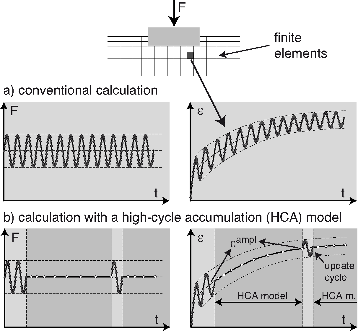
A cyclic loading with an amplitude of \(20\) kPa and \(10^5\) cycles is studied in the following using the high-cycle accumulation (HCA) model. The calculation strategy of the HCA model according to Niemunis et al.1 is illustrated in the figure below.
For the low-cycle phase of the HCA model, the elastic material definition of the previous simulations is kept. For the HCA model the parameters calibrated for "Karlsruhe fine sand" are adopted. The parameters are provided in the table below.
| \(C_{\textrm{ampl}}\) | \(C_{e}\) | \(C_{p}\) | \(C_{Y}\) | \(C_{N1}\) | \(C_{N2}\) | \(C_{N3}\) |
|---|---|---|---|---|---|---|
| 1.33 | 0.60 | 0.23 | 1.68 | 2.95\(\cdot10^{-4}\) | 0.41 | \(1.9 \cdot 10^{-5}\) |
The material definition has to be changed in order to use the HCA model:
*material, name = soil, phases = 2
*Mechanical = HCA_Linear_Elasticity
10000, 0.3
** HCA parameters for Karlsruhe fine sand
**CN1, CN2, CN3, Campl, Ce, 0, Cp2, 0
**Cy2, Cpi1, Cpi2, Cpi3, patm, eref, eps^ampl_ref, A
**a, n, nu, phic
0.000295, 0.41, 0.000019, 1.33, 0.6, 0, 0.23, 0
1.68, 0, 0, 0, 100, 1.0, 0.0001, 1209
1.63, 0.5, 0.32, 0.577

*Implicit hca steps
step1,step2
*Recording hca steps
step3
*Explicit hca steps
step4
*HCA cycle time
1
In addition to the material parameters, the HCA model requires the declaration of the step types. The first two steps are low-cycle ("implicit") steps. The sinusoidal load is applied in step3. The HCA phase is performed in step4. The period of the cycles is 1 s, for why the cycle time is set to 1 s.
Since the HCA model considers the void ratio as a state variable, it has to be initialized. A user file is used, which is the same file as used in the example here. A linearly increasing initial relative density with increasing depth (\(d\)) below the ground surface is defined in this file.
*Initial conditions, type=state variables, user
Soil.all
Warning
If you do not have a fortran compiler available, you can not use user routines. The void ratio has to be defined in the input file in this case, e.g.:
*Initial conditions, type=state variables, default
Soil.all, void_ratio, 0.75
To apply the cyclic loading, a sinusoidal amplitude is defined:
*Amplitude, name = sinus, type = periodic
1,         0,              0.,              6.28
0.,              1.
The steps 3 and 4 are defined as follows.
**
** Load step 3: cyclic loading
**

*Step, name=step3, inc = 10000
*Transient
0.05,1.0,0.0001,0.05

*Body force, instant
Soil.all, GRAV, 9.99, 0, -1, 0
*Body force, instant
Foundation.all, GRAV, 9.99, 0, -1, 0

*Boundary
Foundation.left, u1, 0.0d0
Soil.left,u1,0.0d0
Soil.right,u1,0.0d0
Soil.bottom,u2,0.0d0
Soil.top,pw,0.0d0

*DSload, instant
surf_foundation_top, p, -100.0d0

*DSload, amplitude = sinus
surf_foundation_top, p, -20.0d0

*Controls, global, deactivate
*Controls, u, activate

*Output, field, vtk, ASCII
*Node output, nset = Soil.all
U, pw
*Element output, elset = Soil.all
S, Contact

*Output,print
*frequency = 1
*Node output, nset = Foundation.top_left_node
U

*End Step

**
** Load step 4: HCA phase
**

*Step, name=step4, inc = 10000
*Transient
0.05,1d5,0.0001,5d3

*Body force, instant
Soil.all, GRAV, 9.99, 0, -1, 0
*Body force, instant
Foundation.all, GRAV, 9.99, 0, -1, 0

*Boundary
Foundation.left, u1, 0.0d0
Soil.left,u1,0.0d0
Soil.right,u1,0.0d0
Soil.bottom,u2,0.0d0
Soil.top,pw,0.0d0

*DSload, instant
surf_foundation_top, p, -100.0d0

*Controls, global, deactivate
*Controls, u, activate

*Output, field, vtk, ASCII
*frequency = 25
*Node output, nset = Soil.all
U, pw
*Element output, elset = Soil.all
S, Contact, strain_ampl, void_ratio

*Output,print
*frequency = 1
*Node output, nset = Foundation.top_left_node
U
*End Step

*End input
In step3 the first cycle is applied. The HCA simulation is performed in step4. A total time of \(10^5\) s is defined for the HCA phase. Since each cycle has a period of 1 s, \(10^5\) cycles are simulated. Note that no sinusoidal load is active in step4, only the average loading is applied. The strain amplitude is demanded as output. The field of the strain amplitude calculated based on the recorded strain path of step 3 is given in Fig. 1. Figure 2 depicts the vertical displacement of the foundation vs. time (equivalent to number of load cycles).
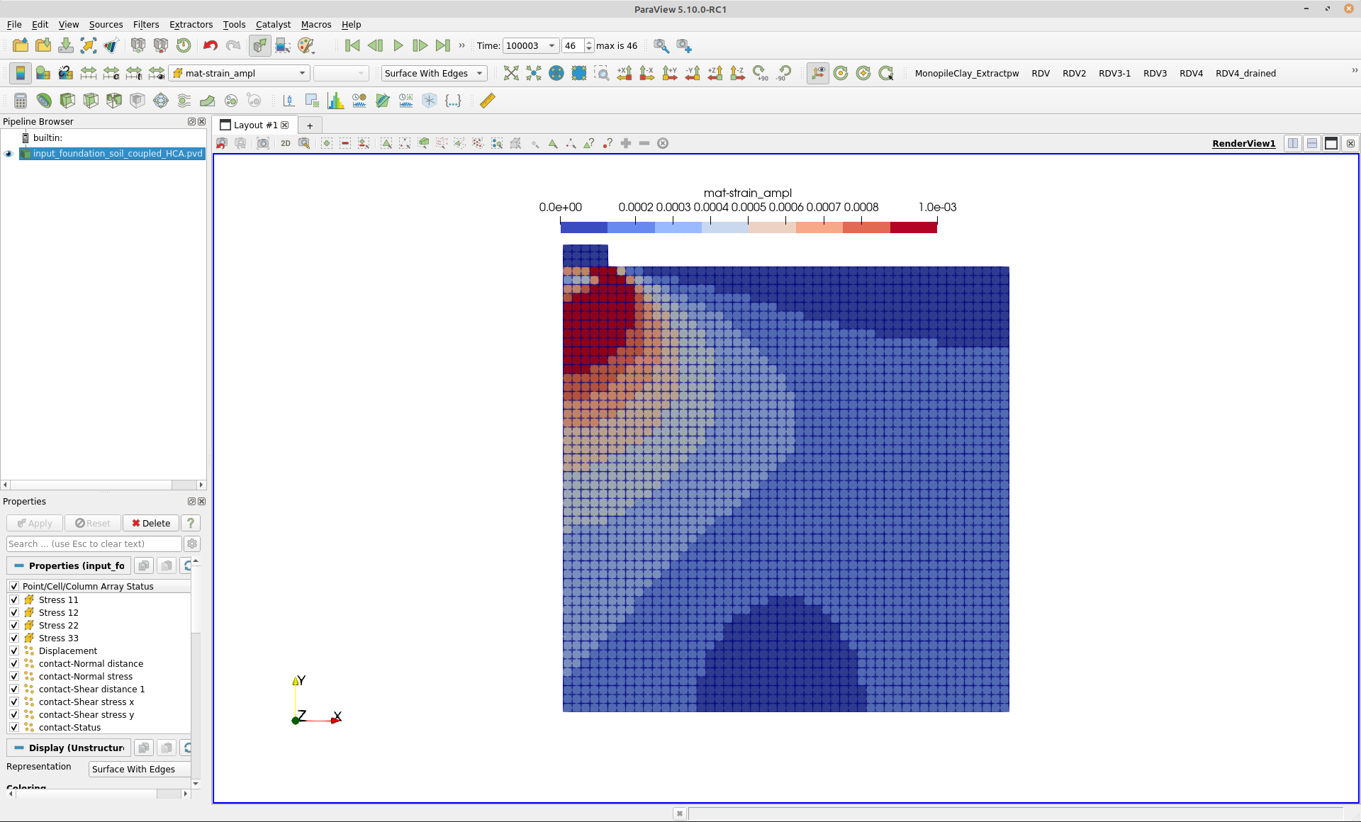 Figure 1. Field of strain amplitude
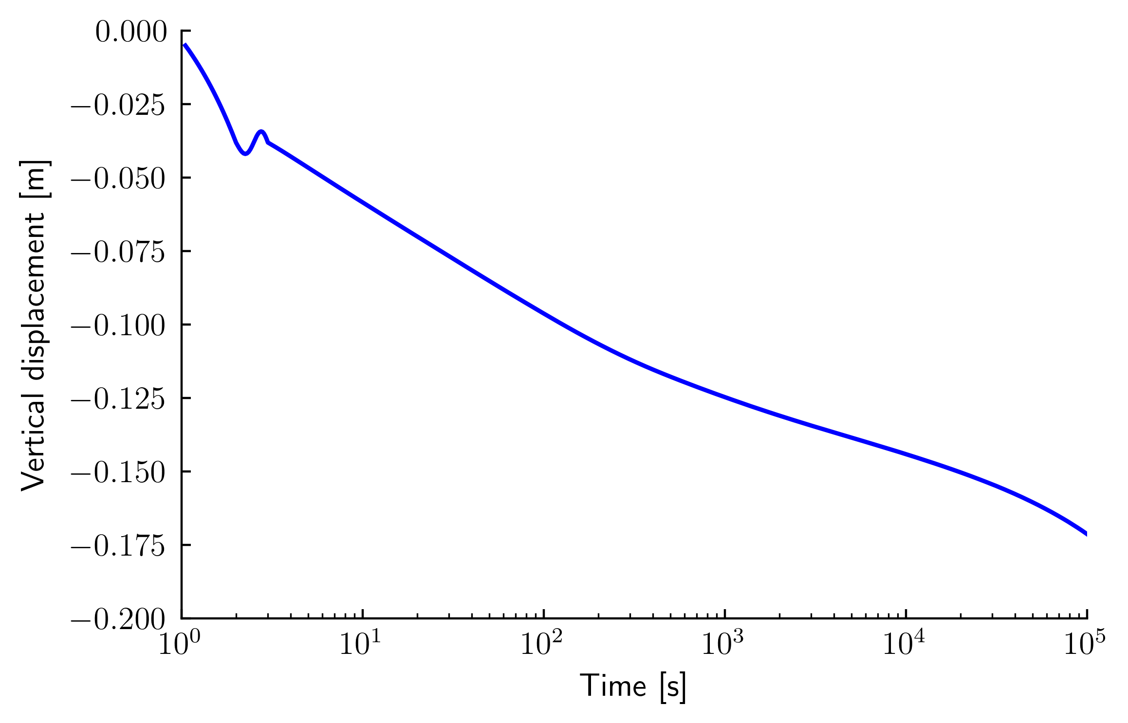 Figure 2. Vertical displacement of the foundation
Python Script for plotting the results
The python script used to generate Figure 2 is given below:
import matplotlib
import matplotlib.pyplot as plt
import matplotlib.ticker as mtick
from pylab import genfromtxt
from matplotlib import rc
import os
dir_path = os.path.dirname(os.path.realpath(__file__))

plt.rcParams['backend'] = "pdf"
plt.rcParams['xtick.direction'] = 'in'
plt.rcParams['ytick.direction'] = 'in'
plt.rcParams['text.usetex'] = True
plt.rcParams['font.size'] = 12
plt.rcParams['axes.spines.right'] = False
plt.rcParams['axes.spines.top'] = False
plt.rcParams['axes.linewidth'] = 0.8

mylinewidth=1.6
mytextwidth=12

mat2 = genfromtxt(dir_path+'/input_foundation_soil_coupled_HCA-print-out/FOUNDATION.TOP_LEFT_NODE_node_7703.dat',skip_header=1);

plt.figure(1)
plt.subplot(111)

plt.semilogx(mat2[:,0], mat2[:,2],'b', linewidth=mylinewidth,\
         markersize=4,markerfacecolor='none',\
         clip_on=True)

ax = plt.gca()

ax.set_xlabel(r'Time [s]',fontsize=mytextwidth)
ax.set_ylabel(r'Vertical displacement [m]',fontsize=mytextwidth,labelpad=7)

ax.axis([1,1e5,-0.2,0])

ax.tick_params(axis='x',direction='in',pad=5,labelsize=mytextwidth)
ax.tick_params(axis='y',direction='in',pad=5,labelsize=mytextwidth)
# ax.grid(True,color='k',linewidth=0.6)

fig = plt.gcf()
fig.savefig('disp_coupled_HCA.pdf', dpi=400 , bbox_inches='tight')
fig.savefig('disp_coupled_HCA.png', dpi=400 , bbox_inches='tight')
-
A Niemunis, T Wichtmann, and T Triantafyllidis. A high-cycle accumulation model for sand. Computers and Geotechnics, 32(4):245–263, 2005. doi:https://doi.org/10.1016/j.compgeo.2005.03.002. ↩