Mono-caisson under high-cyclic loading
Finite Element (FE) representation
Tip
The mesh file for a mono-caisson with a diameter and length of 20 metres and quadratically interpolated elements are found here. The full input files here.
This example explains the simulation of the long-term response of mono-caisson foundations using the HCA model in combination with the hypoplastic model with intergranular strain. The mesh generation is skipped for this example.
Tip
If you are interested you will find more mesh files with other diameters here. Note that the loads in the supplied input file must be adjusted accordingly.
The generated finite element model is shown in Figure 1, the whole model has a radius of 95 m and a depth of 100 m. The mono-caisson is shown with a diameter of 20 m and a length of 20 m. Given the symmetry properties of the foundation structure and the load, it is sufficient to model only half of the mono-caisson and the soil in the simulation, thereby reducin the computational effort. The finite element model employed in this example comprises approximately 3000 elements.
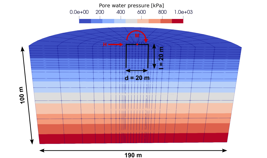 Figure 1. Model of the mono-caisson (only the corner nodes of the elements are visible)
Running out of RAM
The simulation needs quite a bit of RAM. If your simulation is killed, the RAM of your computer is not enough.
Mesh
The definitions of the elements used correspond to the exampel of
the monopile. For the soil, three-dimensional u-p finite elements
with 20 nodes discretising the displacement u of the solid phase
and 8 nodes discretising the pore water pressure \(p^w\) are utilised
(termed u20p8 element).
*Element, type=u20p8-sat
Hence, quadratic interpolation functions are used for the solid displacement while linear interpolation functions are applied for the pore water pressure (i.e. Taylor-Hood element formulation 1).
The mono-caisson is modelled with single phase elements with 20 nodes
(u20-solid).
*Element, type=u20-solid
Material parameters, Contact conditions, Initial conditions and Amplitudes
At the beginning of the input file the mesh.inp-file with the following entry is inserted
*include=mesh_20_20
Material parameters
The material parameters for the steel of the mono-caisson are integrated in the input file as follows. Note that the dead weight of the foundation structure is considered as an external load and therefore a low value is assumed for the density of the steel (0.1 kg/m\(^3\)). In addition, the modulus of elasticity is increased by a factor of \(10^4\), which eliminates the possibility of any inherent deformation of the caisson due to local loads. This assumption is based on the premise that the focus of this simulation is not on the steel structure itself, but rather on the interaction between the mono caisson and the ground under cyclic loading. Finally, the Poisson's ratio of the steel is added.
*Material, Name=Elastisch_Stahl, Phases=1
*Density
0.1d0
** Young's modulus in [kPa], Poisson's ratio
*Mechanical= Linear_Elasticity
2.1e+12, 0.3
The soil of the model is fully saturated with water, resulting in a solid and liquid phase that must be incorporated into the input file. The required material parameters of the "Karlsruhe fine sand" for the low cycle phase calculations of the HCA model, in conjunction with hypoplasticity and intergranular strain extension, are then incorporated 2. Given that the soil is modelled in two phases, it is necessary to specify both the grain density of the "Karlsruhe fine sand" and the water content. In order to prevent the occurrence of tensile stresses, a minimum pressure of -0.01 kPa is established for the entirety of the model. The utilization of the command "Mechanical viscosity" facilitates the incorporation of an artificial viscosity, which results in enhanced numerical calculation stability in instances of rapidly occurring deformations. Nevertheless, the last two entries are not indispensable and do not affect the outcome. The compression modulus of the water is expressed by the bulk modulus. Moreover, the permeability of the soil must be defined. This is achieved by entering the permeability, as indicated by the permeability coefficient of the soil (\(k^w\), assumed to be \(10^{-5}\) m/s), multiplied by the dynamic viscosity of water (\(\eta^w = 10^{-6}\) kPa), divided by the weight of water (\(\gamma_w = 10~\)kN/m\(^3\)) and the dynamic viscosity of the water.
*Material, Name=wo1, Phases=2
*Mechanical=HCA_Hypoplasticity
** Values for hypoplasticity with the addition of intergranular strain
**phi, nu,   h_s,     n,   e_d0,  e_c0,f_ei0,alpha
0.578,0.0,4000000,0.27,0.677,1.054,1.15,0.14
**beta, m_T,m_R, R,  betaR,chi, K^w
2.5,1.2,2.4,0.0001,0.1,6.0, 0.0
**Values for HCA model
** CN1,     CN2,     CN3,     Campl,     Ce,  -,    Cp,    -
0.000295, 0.41, 0.000019,  1.33,    0.6,  0,  0.23, 0.0
** CY, CPi1, CPi2,  CPi3,  pref, eref=emax, epsamplref,   A
1.68, 0.0,  0.0,  0.0, 100.0, 1.054,     0.0001, 1209.0
** a,   n,    nu_HCA,  phi_cc,   -,    -,     -
1.63, 0.50,  0.32,  0.578
**
*Density
2.65d0,1.0d0
**
*Min pressure
-0.01
**
*Mechanical viscosity=linear
0.5,2.0,1.1,1.5,1.1,1.5
**
*Bulk modulus
2.2d6
**
*Permeability=isotropic
1d-12
**
*Dynamic viscosity
1.0e-6
Once the material parameters have been assigned, the calculation steps of the HCA model are assigned. The initial five load steps are calculated in low-cycle mode. In the fifth step, the strain path \(\varepsilon(t)\) is recorded, which serves as the basis for the sixth loading step in high-cycle mode, which constitutes the actual HCA phase.
*Implicit hca steps
step_1,step_2,step_3,step_4
*Recording hca steps
step_5
*Explicit hca steps
step_6
*HCA cycle time
10
Contact conditions
The following section defines the contact conditions between the surfaces of the caisson, its lid, and the soil. This is essential for defining the interaction behavior of the two model components with the soil. The penalty method is employed to ensure the enforcement of the contact constraints. Upon issuing the "no separation" command, the contact surfaces are coupled together in such a way that they can no longer be separated from each other after a single contact. A simple Coulomb friction model with a friction coefficient of 0.405 is employed to facilitate controlled interaction between the elements. Contact between the soil and the pile is discretized using a mortar contact discretization method. Contact conditions are transferred by defining the respective contact pairs. To optimize the contact conditions, the clearance option is introduced, enabling the distance between the contact pairs in the contact zone to be determined. Positive values indicate an open contact, while negative values indicate an overlap.
*Interaction,Name=pen,Mechanical=penalty,no separation,stiffness_factor=20,non constant
*Friction,model=MC
4e3,0.405,0,0
**
*Contact pair,Interaction=pen,Discretisation=element mortar
BodenMonopileAussenSurface,MonopileAussenSurface
BodenMonopileInnenSurface,MonopileInnenSurface
BodenPfahlfussSurface,MonopileUntenSurface
PfahlkopfUntenInnenSurface,BodenPfahlkopfObenInnenS1Surface
**
*Contact options,Name=pen,clearance=1d-6
Initial conditions
The initial conditions define the initial states of the soil in terms of the pore number \(e\), the effective initial stresses of the soil \(\sigma′\) and the initial pore water pressure \(p_w\). The void ratio \(e\) is given by \(e\) = \(e_{max}\) - \(I_{D0}\) \(\cdot\) (\(e_{max}\) - \(e_{min}\)) . Furthermore, the intergranular strain is entered in the z-direction with a maximum value of \(R\) = \(-10^{-4}\). The effective initial stress of the soil is given by, \(\sigma′\) = \(\gamma'\) \(\cdot\) \(z\) and the effective initial pore water pressure \(p_w\) = \(\gamma_w\) \(\cdot\) \(z\).
It is also necessary to consider the additional compressive stress \(\sigma′_A\), which is applied to the entire top edge of the floor in the subsequent loading stages. This serves to stabilise the numerical calculation and is added to the initial stress of the floor, \(\sigma′\).
*Initial conditions,Type=void ratio,default
BodenInstance.BodenAlle,0.7524d0
**
*Initial conditions,Type=state variables,default
Geometrie_Bodenkoerper_Aussen4,void_ratio,0.7524d0
Geometrie_Bodenkoerper_Aussen5,void_ratio,0.7524d0
Geometrie_Bodenkoerper_Innen4,void_ratio,0.7524d0
Geometrie_Bodenkoerper_Aussen4,int_strain33,-0.0001
Geometrie_Bodenkoerper_Aussen5,int_strain33,-0.0001
Geometrie_Bodenkoerper_Innen4,int_strain33,-0.0001
**
*Initial conditions,Type=stress,Geostatic
BodenInstance.BodenAlle,0,-5,100,-946.6,0.452,0.452
**
*Initial conditions, Type=pore water pressure,default
BodenInstance.BodenAlle,0.0d0,0d0,100.0d0,1000.0d0
Amplitudes
To calculate the load steps, it is necessary to define the load amplitudes. These are needed to define the course of the load applied to the model. The amplitude \(LoadingRamp\) with the specified ramp type represents the rate at which the load increases linearly over the specified loading period. The initial time point, designated \(t_1=0\), is defined as the point at which no load is applied. Conversely, the final time point, designated \(t_2=1\), is defined as the point at which the full load is applied. Furthermore, a sinusoidal load application with a frequency of 0.1 Hz (\(\omega\) = 0.628 rad/s) has been selected for the cyclic load. A frequency of 0.1 Hz has a period length of T = 10 s, where the period length indicates the duration of the load cycle in physical time. A load frequency of 0.1 Hz represents typical conditions in the North Sea, while a frequency of 1 Hz represents an extreme case.
*Amplitude,Name=LoadingRamp,Type=ramp
0.0,0.0,1.0d0,1.0d0
*Amplitude,Name=Sinus0_1Hz,Type=periodic
1,0.0,0.0,0.628
0,1
Steps and loading definitions
The simulation of the high-cycle load is conducted in a series of discrete steps, each of which is designed to fulfill a specific function that is necessary for calculating the load history. In the present example, six load steps are required, which are explained below.
Step 1
In the first step, the dead weight of the soil and the mono-caisson is applied to the model. For this purpose, the Geostatic
analysis method is selected and the model is brought into equilibrium by applying the gravitational forces in the z-direction.
The acceleration due to gravity \(g\) is assumed to be \(10\) m/s\(^2\). In addition, a compressive stress of 5 kPa is applied to the surface
of the ground to improve the numerical calculation stability. This is to prevent the occurrence of tensile stresses at the top edge
of the soil. All nodal points of the model, as well as the pore water pressure, are restrained by boundaries in all directions
(x-, y- and z-direction), so that no displacements can occur. Since the mono-caisson is modeled by two individual segments,
the jacket and the cover, it must be ensured that these do not separate as a result of the simulation, an immovable connection
of both segments in all displacement directions is created with the help of Equation. The error controls are deactivated at
global level, but it is activated in the default setting for the solid displacement \(u\)). The output is in vtk format (suitable for ParaView)
and is of type ASCII. The node output contains the displacement (U) and the pore water pressure (PW) of the nodes. The element
output contains the stress (S) as well as the void ratio (Void_ratio) and the contact output variables (Contact). The contact
output contains the contact stresses and the contact distances for each contact node.
****------------------------------Step 1:--------------------------------
** Deadweight of the soil
*Step,Name=step_1,inc=1
*Geostatic
**
**--------------------------------Load-----------------------------------
** Gravity (1g)
*Body force,instant
BodenInstance.BodenAlle,Grav,10,0.0,0.0,1.0
*Body force,instant
MonopileInstance.MonopileAlle,Grav,10,0.0,0.0,1.0
*Body force,instant
PfahlkopfInstance.PfahlkopfAlle,Grav,10,0.0,0.0,1.0
**
**---------------Low load to stabilize the calculation 5kPa--------------
**
*Dload, instant
_BodenObenS1Surface_S2,P2,-5.d0
*Dload,instant
_BodenObenS1Surface_S3,P3,-5.d0
**
**------------------------------Boundary---------------------------------
**
*Boundary
MonopileInstance.MonopileAlle,u1,0.0d0
MonopileInstance.MonopileAlle,u2,0.0d0
MonopileInstance.MonopileAlle,u3,0.0d0
PfahlkopfInstance.PfahlkopfAlle,u1,0.0d0
PfahlkopfInstance.PfahlkopfAlle,u2,0.0d0
PfahlkopfInstance.PfahlkopfAlle,u3,0.0d0
BodenInstance.BodenAlle,u1,0.0d0
BodenInstance.BodenAlle,u2,0.0d0
BodenInstance.BodenAlle,u3,0.0d0
**
*Boundary,hydrostatic
BodenInstance.BodenAlle,pw,10.0d0,0.0d0
**
**-----------Non-displaceable connection from jacket to cover------------
**
*Equation
Knoten_Monopile_Aussen_Oben_Links,u1,Knoten_Pfahlkopf_Aussen_Unten_Links,u1
*Equation
Knoten_Monopile_Aussen_Oben_Links,u2,Knoten_Pfahlkopf_Aussen_Unten_Links,u2
*Equation
Knoten_Monopile_Aussen_Oben_Links,u3,Knoten_Pfahlkopf_Aussen_Unten_Links,u3
*Equation
Knoten_Monopile_Aussen_Oben_Rechts,u1,Knoten_Pfahlkopf_Aussen_Unten_Rechts,u1
*Equation
Knoten_Monopile_Aussen_Oben_Rechts,u2,Knoten_Pfahlkopf_Aussen_Unten_Rechts,u2
*Equation
Knoten_Monopile_Aussen_Oben_Rechts,u3,Knoten_Pfahlkopf_Aussen_Unten_Rechts,u3
*Equation
Knoten_Monopile_Innen_Oben_Links,u1,Knoten_Pfahlkopf_Innen_Unten_Links,u1
*Equation
Knoten_Monopile_Innen_Oben_Links,u2,Knoten_Pfahlkopf_Innen_Unten_Links,u2
*Equation
Knoten_Monopile_Innen_Oben_Links,u3,Knoten_Pfahlkopf_Innen_Unten_Links,u3
*Equation
Knoten_Monopile_Innen_Oben_Rechts,u1,Knoten_Pfahlkopf_Innen_Unten_Rechts,u1
*Equation
Knoten_Monopile_Innen_Oben_Rechts,u2,Knoten_Pfahlkopf_Innen_Unten_Rechts,u2
*Equation
Knoten_Monopile_Innen_Oben_Rechts,u3,Knoten_Pfahlkopf_Innen_Unten_Rechts,u3
**
**------------------------------Controls---------------------------------
*Controls,global,deactivate
*Controls,u,activate
**
**-------------------------------Output----------------------------------
**
*Output,field,vtk,ascii
*Node output,nset=BodenInstance.BodenAlle
U,Pw
*Element output, elset=BodenInstance.BodenAlle
S,Contact,Contact_diagnostic,proj,void_ratio
**
*Output,print
**
*Node output,nset=Knoten_Pfahlkopf_Aussen_Oben_Links
U
*Node output,nset=Knoten_Pfahlkopf_Aussen_Oben_Rechts
U
*Node output,nset=Knoten_Pfahlkopf_Mitte_Oben
U
**
*Node output,nset=Node_BodenOben_Mitte
Pw, coords
*Node output,nset=Node_BodenUnten_Links
Pw, coords
*Node output,nset=Node_BodenUnten_Rechts
Pw, coords

*End Step
Step 2
In the second step, the dead weight of the foundation structure and the wind turbine is applied to the top of the mono-caisson. The assumed
weight is 3,097 tons. A static analysis method is selected which neglects inertia effects. The load from the dead weight is applied to the
model in full with the command Dload and the addition instant without any time delay. In this example, the size of the load is 49.3 kPa.
The boundary conditions are adjusted so that the model is only held normally at its edges, allowing the dead weight to act freely. The pore
water pressure, on the other hand, is still held hydrostatically.
****------------------------------Step 2:--------------------------------
** Weight of the wind turbine
*Step,Name=step_2,inc=100,maxiter=6
*Static
1,1,0.0001,1
**
**--------------------------------Load-----------------------------------
** Gravity (1g)
*Body force,instant
BodenInstance.BodenAlle,Grav,10,0.0,0.0,1.0
*Body force,instant
MonopileInstance.MonopileAlle,Grav,10,0.0,0.0,1.0
*Body force,instant
PfahlkopfInstance.PfahlkopfAlle,Grav,10,0.0,0.0,1.0
**
**---------------Low load to stabilize the calculation 5kPa--------------
**
*Dload, instant
_BodenObenS1Surface_S2,P2,-5.d0
*Dload,instant
_BodenObenS1Surface_S3,P3,-5.d0
**
**--------------------Load of the wind turbine in kpa/m2-----------------
**
*Dload,instant
_PfahlkopfObenSurfaceMonopile_S2,P2,-49.3
**
**------------------------------Boundary---------------------------------
**
*Boundary
Boden_Hinten,u1,0.0d0
Boden_Hinten,u2,0.0d0
Boden_Unten_S5,u3,0.0d0
Boden_Symmetrie_Vorne_Links,u2,0.0d0
Boden_Symmetrie_Vorne_Mitte,u2,0.0d0
Boden_Symmetrie_Vorne_Rechts,u2,0.0d0
Monopile_Symmetrie_Vorne,u2,0.0d0
Pfahlkopf_Symmetrie_Vorne,u2,0.0d0
**
*Boundary,hydrostatic
BodenInstance.BodenAlle,pw,10.0d0,0.0d0
**
**-----------Non-displaceable connection from jacket to cover------------
**
*Equation
Knoten_Monopile_Aussen_Oben_Links,u1,Knoten_Pfahlkopf_Aussen_Unten_Links,u1
*Equation
Knoten_Monopile_Aussen_Oben_Links,u2,Knoten_Pfahlkopf_Aussen_Unten_Links,u2
*Equation
Knoten_Monopile_Aussen_Oben_Links,u3,Knoten_Pfahlkopf_Aussen_Unten_Links,u3
*Equation
Knoten_Monopile_Aussen_Oben_Rechts,u1,Knoten_Pfahlkopf_Aussen_Unten_Rechts,u1
*Equation
Knoten_Monopile_Aussen_Oben_Rechts,u2,Knoten_Pfahlkopf_Aussen_Unten_Rechts,u2
*Equation
Knoten_Monopile_Aussen_Oben_Rechts,u3,Knoten_Pfahlkopf_Aussen_Unten_Rechts,u3
*Equation
Knoten_Monopile_Innen_Oben_Links,u1,Knoten_Pfahlkopf_Innen_Unten_Links,u1
*Equation
Knoten_Monopile_Innen_Oben_Links,u2,Knoten_Pfahlkopf_Innen_Unten_Links,u2
*Equation
Knoten_Monopile_Innen_Oben_Links,u3,Knoten_Pfahlkopf_Innen_Unten_Links,u3
*Equation
Knoten_Monopile_Innen_Oben_Rechts,u1,Knoten_Pfahlkopf_Innen_Unten_Rechts,u1
*Equation
Knoten_Monopile_Innen_Oben_Rechts,u2,Knoten_Pfahlkopf_Innen_Unten_Rechts,u2
*Equation
Knoten_Monopile_Innen_Oben_Rechts,u3,Knoten_Pfahlkopf_Innen_Unten_Rechts,u3
**
**------------------------------Controls---------------------------------
**
*Controls,global,deactivate
*Controls,u,activate
**
**-------------------------------Output----------------------------------
**
*Output,field,vtk,ascii
*Node output,nset=BodenInstance.BodenAlle
U,Pw
*Element output,elset=BodenInstance.BodenAlle
S,Contact,Contact_diagnostic,proj,void_ratio
**
*Output, print
**
*Node output,nset=Knoten_Pfahlkopf_Aussen_Oben_Links
U
*Node output,nset=Knoten_Pfahlkopf_Aussen_Oben_Rechts
U
*Node output,nset=Knoten_Pfahlkopf_Mitte_Oben
U
**
*Node output,nset=Node_BodenOben_Mitte
Pw, coords
*Node output,nset=Node_BodenUnten_Links
Pw, coords
*Node output,nset=Node_BodenUnten_Rechts
Pw, coords

*End Step
Step 3
In the third step, the mean value of the cyclic load is applied to the model. Similarly, the static analysis method is selected for this
purpose. The mean value of the cyclic load is composed of a horizontal component (\(H\)) and a moment component (\(M\)). The moment is applied
by a vertically acting force pair (\(V\)) with points of application on the left and right of the outer points of the mono-caisson cover ($5906,25\cdot10\cdot2 = 118,125 MNm).
It should be noted that due to the symmetry properties of the model, the applied loads must be halved, as only half of the model has been modelled.
The mean value of the load is applied linearly increasing to a defined node set with the previously introduced amplitude \(LoadingRamp\) using the
command Cload. Finally, the Controls command is used to influence the severity of the convergence criteria.
****------------------------------Step 3:--------------------------------
** Monotone load from wind and waves
*Step,Name=step_3,inc=5000
*Static
0.05,1.0d0,0.0001,0.05
**
**--------------------------------Load-----------------------------------
** Gravity (1g)
*Body force,instant
BodenInstance.BodenAlle,Grav,10,0.0,0.0,1.0
*Body force,instant
MonopileInstance.MonopileAlle,Grav,10,0.0,0.0,1.0
*Body force,instant
PfahlkopfInstance.PfahlkopfAlle,Grav,10,0.0,0.0,1.0
**
**---------------Low load to stabilize the calculation 5kPa--------------
**
*Dload, instant
_BodenObenS1Surface_S2,P2,-5.d0
*Dload,instant
_BodenObenS1Surface_S3,P3,-5.d0
**
**--------------------Load of the wind turbine in kpa/m2-----------------
**
*Dload,instant
_PfahlkopfObenSurfaceMonopile_S2,P2,-49.3
**
**--------------------Load from wind and waves MONO ---------------------
** M_ult = 675 MNm
*Cload,amplitude=LoadingRamp
Knoten_Pfahlkopf_Aussen_Oben_Links,1,-328.1
*Cload,amplitude=LoadingRamp
Knoten_Pfahlkopf_Aussen_Oben_Rechts,1,-328.1
*Cload,amplitude=LoadingRamp
Knoten_Pfahlkopf_Aussen_Oben_Links,3,-1968.75
*Cload,amplitude=LoadingRamp
Knoten_Pfahlkopf_Aussen_Oben_Rechts,3,1968.75
**
**------------------------------Boundary---------------------------------
**
*Boundary
Boden_Hinten,u1,0.0d0
Boden_Hinten,u2,0.0d0
Boden_Unten_S5,u3,0.0d0
Boden_Symmetrie_Vorne_Links,u2,0.0d0
Boden_Symmetrie_Vorne_Mitte,u2,0.0d0
Boden_Symmetrie_Vorne_Rechts,u2,0.0d0
Monopile_Symmetrie_Vorne,u2,0.0d0
Pfahlkopf_Symmetrie_Vorne,u2,0.0d0
**
*Boundary,hydrostatic
BodenInstance.BodenAlle,pw,10.0d0,0.0d0
**
**-----------Non-displaceable connection from jacket to cover------------
**
*Equation
Knoten_Monopile_Aussen_Oben_Links,u1,Knoten_Pfahlkopf_Aussen_Unten_Links,u1
*Equation
Knoten_Monopile_Aussen_Oben_Links,u2,Knoten_Pfahlkopf_Aussen_Unten_Links,u2
*Equation
Knoten_Monopile_Aussen_Oben_Links,u3,Knoten_Pfahlkopf_Aussen_Unten_Links,u3
*Equation
Knoten_Monopile_Aussen_Oben_Rechts,u1,Knoten_Pfahlkopf_Aussen_Unten_Rechts,u1
*Equation
Knoten_Monopile_Aussen_Oben_Rechts,u2,Knoten_Pfahlkopf_Aussen_Unten_Rechts,u2
*Equation
Knoten_Monopile_Aussen_Oben_Rechts,u3,Knoten_Pfahlkopf_Aussen_Unten_Rechts,u3
*Equation
Knoten_Monopile_Innen_Oben_Links,u1,Knoten_Pfahlkopf_Innen_Unten_Links,u1
*Equation
Knoten_Monopile_Innen_Oben_Links,u2,Knoten_Pfahlkopf_Innen_Unten_Links,u2
*Equation
Knoten_Monopile_Innen_Oben_Links,u3,Knoten_Pfahlkopf_Innen_Unten_Links,u3
*Equation
Knoten_Monopile_Innen_Oben_Rechts,u1,Knoten_Pfahlkopf_Innen_Unten_Rechts,u1
*Equation
Knoten_Monopile_Innen_Oben_Rechts,u2,Knoten_Pfahlkopf_Innen_Unten_Rechts,u2
*Equation
Knoten_Monopile_Innen_Oben_Rechts,u3,Knoten_Pfahlkopf_Innen_Unten_Rechts,u3
**
**------------------------------Controls---------------------------------
**
*Controls,global,deactivate
*Controls,u,modify
0.03,0.03,0.02,1d-9,1d-9,2
**
**-------------------------------Output----------------------------------
**
*Output,field,vtk,ascii
*Frequency=5
*Node output,nset=BodenInstance.BodenAlle
U,Pw
*Element output,elset=BodenInstance.BodenAlle
S,Contact,Contact_diagnostic,proj,void_ratio
**
*Output,print
**
*Node output,nset=Knoten_Pfahlkopf_Aussen_Oben_Links
U
*Node output,nset=Knoten_Pfahlkopf_Aussen_Oben_Rechts
U
*Node output,nset=Knoten_Pfahlkopf_Mitte_Oben
U
**
*Node output,nset=Node_BodenOben_Mitte
Pw, coords
*Node output,nset=Node_BodenUnten_Links
Pw, coords
*Node output,nset=Node_BodenUnten_Rechts
Pw, coords

*End Step
Step 4 and Step 5
The fourth and fifth steps are identical, differing only in their nomenclature. Both steps are calculated in low-cycle mode.
The previously applied mean value is augmented by the introduction of a sinusoidal load. A transient analysis method is selected that
enables the calculation according to physical time. The sinusoidal load is applied to the same nodes as the previously defined mean value.
The utilisation of physical time is imperative in this phase, as it facilitates the temporal alteration of the free pore water pressure
throughout the entire model. In order to achieve this, the boundary conditions for the pore water pressure outside the edges of the model
are released. This enables the inflow and outflow of pore water from above, below and behind, as well as the build-up of excess or
negative pore water pressure in the model. The other boundary conditions remain unchanged. Furthermore, the convergence criteria are
supplemented and not changed in the further steps of the calculation.
A recalculation of the fourth step is required because the strain path \(\varepsilon(t)\) can only be recorded in the fifth step. At the conclusion of this step, the strain amplitude \(\varepsilon_{ampl}\) is calculated and serves as the basis for the subsequent simulation of the HCA phase. It is only possible to demonstrate the strain path \(\varepsilon(t)\) in step 5, as an initial loading of the soil occurs in the initial quarter of step 4, which results in a peak value with a larger permanent deformation. Such deformation would then be transferred to all subsequent cycles.
****------------------------------Step 4:--------------------------------
** first cycle in the hypoplastic model
*Step,Name=step_4,inc=10000
*Transient
0.5,10.0,0.01,0.5
**
**
**--------------------------------Load-----------------------------------
** Gravity (1g)
*Body force,instant
BodenInstance.BodenAlle,Grav,10,0.0,0.0,1.0
*Body force,instant
MonopileInstance.MonopileAlle,Grav,10,0.0,0.0,1.0
*Body force,instant
PfahlkopfInstance.PfahlkopfAlle,Grav,10,0.0,0.0,1.0
**
**---------------Low load to stabilize the calculation 5kPa--------------
**
*Dload, instant
_BodenObenS1Surface_S2,P2,-5.d0
*Dload,instant
_BodenObenS1Surface_S3,P3,-5.d0
**
**--------------------Load of the wind turbine in kpa/m2-----------------
**
*Dload,instant
_PfahlkopfObenSurfaceMonopile_S2,P2,-49.3
**
**--------------------Load from wind and waves MONO ---------------------
**
*Cload,instant
Knoten_Pfahlkopf_Aussen_Oben_Links,1,-328.1
*Cload,instant
Knoten_Pfahlkopf_Aussen_Oben_Rechts,1,-328.1
*Cload,instant
Knoten_Pfahlkopf_Aussen_Oben_Links,3,-1968.75
*Cload,instant
Knoten_Pfahlkopf_Aussen_Oben_Rechts,3,1968.75
**
**------------------Load from wind and waves cyclical--------------------
**
*Cload,amplitude=Sinus0_1Hz
Knoten_Pfahlkopf_Aussen_Oben_Links,1,-328.1
*Cload,amplitude=Sinus0_1Hz
Knoten_Pfahlkopf_Aussen_Oben_Rechts,1,-328.1
*Cload,amplitude=Sinus0_1Hz
Knoten_Pfahlkopf_Aussen_Oben_Links,3,-1968.75
*Cload,amplitude=Sinus0_1Hz
Knoten_Pfahlkopf_Aussen_Oben_Rechts,3,1968.75
**
**------------------------------Boundary---------------------------------
**
*Boundary
Boden_Hinten,u1,0.0d0
Boden_Hinten,u2,0.0d0
Boden_Unten_S5,u3,0.0d0
Boden_Symmetrie_Vorne_Links,u2,0.0d0
Boden_Symmetrie_Vorne_Mitte,u2,0.0d0
Boden_Symmetrie_Vorne_Rechts,u2,0.0d0
Monopile_Symmetrie_Vorne,u2,0.0d0
Pfahlkopf_Symmetrie_Vorne,u2,0.0d0
**
*Boundary,hydrostatic
Boden_Oben_S1_PWD,pw,10.0d0,0.0d0
Boden_hinten,pw,10.0d0,0.0d0
Boden_Unten_S5,pw,10.0d0,0.0d0
**
**-----------Non-displaceable connection from jacket to cover------------
**
*Equation
Knoten_Monopile_Aussen_Oben_Links,u1,Knoten_Pfahlkopf_Aussen_Unten_Links,u1
*Equation
Knoten_Monopile_Aussen_Oben_Links,u2,Knoten_Pfahlkopf_Aussen_Unten_Links,u2
*Equation
Knoten_Monopile_Aussen_Oben_Links,u3,Knoten_Pfahlkopf_Aussen_Unten_Links,u3
*Equation
Knoten_Monopile_Aussen_Oben_Rechts,u1,Knoten_Pfahlkopf_Aussen_Unten_Rechts,u1
*Equation
Knoten_Monopile_Aussen_Oben_Rechts,u2,Knoten_Pfahlkopf_Aussen_Unten_Rechts,u2
*Equation
Knoten_Monopile_Aussen_Oben_Rechts,u3,Knoten_Pfahlkopf_Aussen_Unten_Rechts,u3
*Equation
Knoten_Monopile_Innen_Oben_Links,u1,Knoten_Pfahlkopf_Innen_Unten_Links,u1
*Equation
Knoten_Monopile_Innen_Oben_Links,u2,Knoten_Pfahlkopf_Innen_Unten_Links,u2
*Equation
Knoten_Monopile_Innen_Oben_Links,u3,Knoten_Pfahlkopf_Innen_Unten_Links,u3
*Equation
Knoten_Monopile_Innen_Oben_Rechts,u1,Knoten_Pfahlkopf_Innen_Unten_Rechts,u1
*Equation
Knoten_Monopile_Innen_Oben_Rechts,u2,Knoten_Pfahlkopf_Innen_Unten_Rechts,u2
*Equation
Knoten_Monopile_Innen_Oben_Rechts,u3,Knoten_Pfahlkopf_Innen_Unten_Rechts,u3
**
**------------------------------Controls---------------------------------
**
*Controls,global,deactivate
*Controls,u,modify
0.07,0.07,0.06,1d-9,1d-9,3
*Controls,pw,deactivate
**
**-------------------------------Output----------------------------------
*Output,field,vtk,ascii
*Frequency=3
*Node output, nset=BodenInstance.BodenAlle
U,Pw
*Element output,elset=BodenInstance.BodenAlle
S,Contact,Contact_diagnostic,proj,void_ratio
**
*Output,print
**
*Node output,nset=Knoten_Pfahlkopf_Aussen_Oben_Links
U
*Node output,nset=Knoten_Pfahlkopf_Aussen_Oben_Rechts
U
*Node output,nset=Knoten_Pfahlkopf_Mitte_Oben
U
**
*Node output,nset=Node_BodenOben_Mitte
Pw,coords
*Node output,nset=Node_BodenUnten_Links
Pw,coords
*Node output,nset=Node_BodenUnten_Rechts
Pw,coords

*End Step
Step 6
In the sixth and final step, the high-cycle load is calculated over a period of \(10^7\) cycles in high-cycle mode. The results can be employed to ascertain the deformations of the soil and the rotation of the wind turbine. In this step, the definition of the cyclic load is omitted, as this is no longer necessary due to the strain amplitude calculated in the previous step. Consequently, the accumulation of displacement resulting from the sinusoidally applied cyclic load can now be determined on the basis of the aforementioned strain amplitude.
****------------------------------Step 6:--------------------------------
** Calculation with HCA model
*Step,Name=step_6,inc=100000
*Transient
0.5,1e7,0.5,1e5
**
*Extrapolation,none
**
**--------------------------------Load-----------------------------------
**
** Gravity (1g)
*Body force,instant
BodenInstance.BodenAlle,Grav,10,0.0,0.0,1.0
*Body force,instant
MonopileInstance.MonopileAlle,Grav,10,0.0,0.0,1.0
*Body force,instant
PfahlkopfInstance.PfahlkopfAlle,Grav,10,0.0,0.0,1.0
**
**---------------Low load to stabilize the calculation 5kPa--------------
**
*Dload, instant
_BodenObenS1Surface_S2,P2,-5.d0
*Dload,instant
_BodenObenS1Surface_S3,P3,-5.d0
**
**--------------------Load of the wind turbine in kpa/m2-----------------
**
*Dload,instant
_PfahlkopfObenSurfaceMonopile_S2,P2,-49.3
**
**--------------------Load from wind and waves MONO ---------------------
**
*Cload,instant
Knoten_Pfahlkopf_Aussen_Oben_Links,1,-328.1
*Cload,instant
Knoten_Pfahlkopf_Aussen_Oben_Rechts,1,-328.1
*Cload,instant
Knoten_Pfahlkopf_Aussen_Oben_Links,3,-1968.75
*Cload,instant
Knoten_Pfahlkopf_Aussen_Oben_Rechts,3,1968.75
**
**------------------------------Boundary---------------------------------
**Schwerkraft (1g)
*Boundary
Boden_Hinten,u1,0.0d0
Boden_Hinten,u2,0.0d0
Boden_Unten_S5,u3,0.0d0
Boden_Symmetrie_Vorne_Links,u2,0.0d0
Boden_Symmetrie_Vorne_Mitte,u2,0.0d0
Boden_Symmetrie_Vorne_Rechts,u2,0.0d0
Monopile_Symmetrie_Vorne,u2,0.0d0
Pfahlkopf_Symmetrie_Vorne,u2,0.0d0
**
*Boundary,hydrostatic
Boden_Oben_S1_PWD,pw,10.0d0,0.0d0
Boden_hinten,pw,10.0d0,0.0d0
Boden_Unten_S5,pw,10.0d0,0.0d0
**
**-----------Non-displaceable connection from jacket to cover------------
**
*Equation
Knoten_Monopile_Aussen_Oben_Links,u1,Knoten_Pfahlkopf_Aussen_Unten_Links,u1
*Equation
Knoten_Monopile_Aussen_Oben_Links,u2,Knoten_Pfahlkopf_Aussen_Unten_Links,u2
*Equation
Knoten_Monopile_Aussen_Oben_Links,u3,Knoten_Pfahlkopf_Aussen_Unten_Links,u3
*Equation
Knoten_Monopile_Aussen_Oben_Rechts,u1,Knoten_Pfahlkopf_Aussen_Unten_Rechts,u1
*Equation
Knoten_Monopile_Aussen_Oben_Rechts,u2,Knoten_Pfahlkopf_Aussen_Unten_Rechts,u2
*Equation
Knoten_Monopile_Aussen_Oben_Rechts,u3,Knoten_Pfahlkopf_Aussen_Unten_Rechts,u3
*Equation
Knoten_Monopile_Innen_Oben_Links,u1,Knoten_Pfahlkopf_Innen_Unten_Links,u1
*Equation
Knoten_Monopile_Innen_Oben_Links,u2,Knoten_Pfahlkopf_Innen_Unten_Links,u2
*Equation
Knoten_Monopile_Innen_Oben_Links,u3,Knoten_Pfahlkopf_Innen_Unten_Links,u3
*Equation
Knoten_Monopile_Innen_Oben_Rechts,u1,Knoten_Pfahlkopf_Innen_Unten_Rechts,u1
*Equation
Knoten_Monopile_Innen_Oben_Rechts,u2,Knoten_Pfahlkopf_Innen_Unten_Rechts,u2
*Equation
Knoten_Monopile_Innen_Oben_Rechts,u3,Knoten_Pfahlkopf_Innen_Unten_Rechts,u3
**
**------------------------------Controls---------------------------------
**
*Controls,global,deactivate
*Controls,u,modify
0.07,0.07,0.06,1d-9,1d-9,3
*Controls,pw,deactivate
**
**-------------------------------Output----------------------------------
**
*Output,field,vtk,ascii
*Frequency=10
*Node output,nset=BodenInstance.BodenAlle
U,Pw
*Element output,elset=BodenInstance.BodenAlle
S,Contact,Contact_diagnostic,Strain_ampl,Strain_acc,cyclic_history,fampl,fe,fp,fY,proj,void_ratio
**
*Output,print
**
*Node output,nset=Knoten_Pfahlkopf_Aussen_Oben_Links
U
*Node output,nset=Knoten_Pfahlkopf_Aussen_Oben_Rechts
U
*Node output,nset=Knoten_Pfahlkopf_Mitte_Oben
U
**
*Node output,nset=Node_BodenOben_Mitte
Pw,coords
*Node output,nset=Node_BodenUnten_Links
Pw,coords
*Node output,nset=Node_BodenUnten_Rechts
Pw,coords

*End Step
**
*End Input
The input file is now complete, thus enabling the commencement of the calculation. To accomplish this, the name of the input file must be entered into the command line (without ending), then confirmed with the Enter key. The number of CPUs to be used must then be added (depending on the hardware, 4 CPUs are appropriated here), and the Enter key must be pressed again to confirm.
Results of the simulation
When the calculation is complete (the command window is ready for a new command), open the .sta file and check if the simulation was successful.
This is indicated by the fact that all steps were completed successfully. If the simulation stops after starting, check the error messages in
the .log file and the error files created in the calculation folder. The input file must be corrected. If the calculation is successful, it is
possible to evaluate it graphically in ParaView. To do so, open the pvd file (in the right upper options bar: "File" \(\rightarrow\)
"Open..."). A possible
graphical evaluation of the example file is shown in Figure 2.
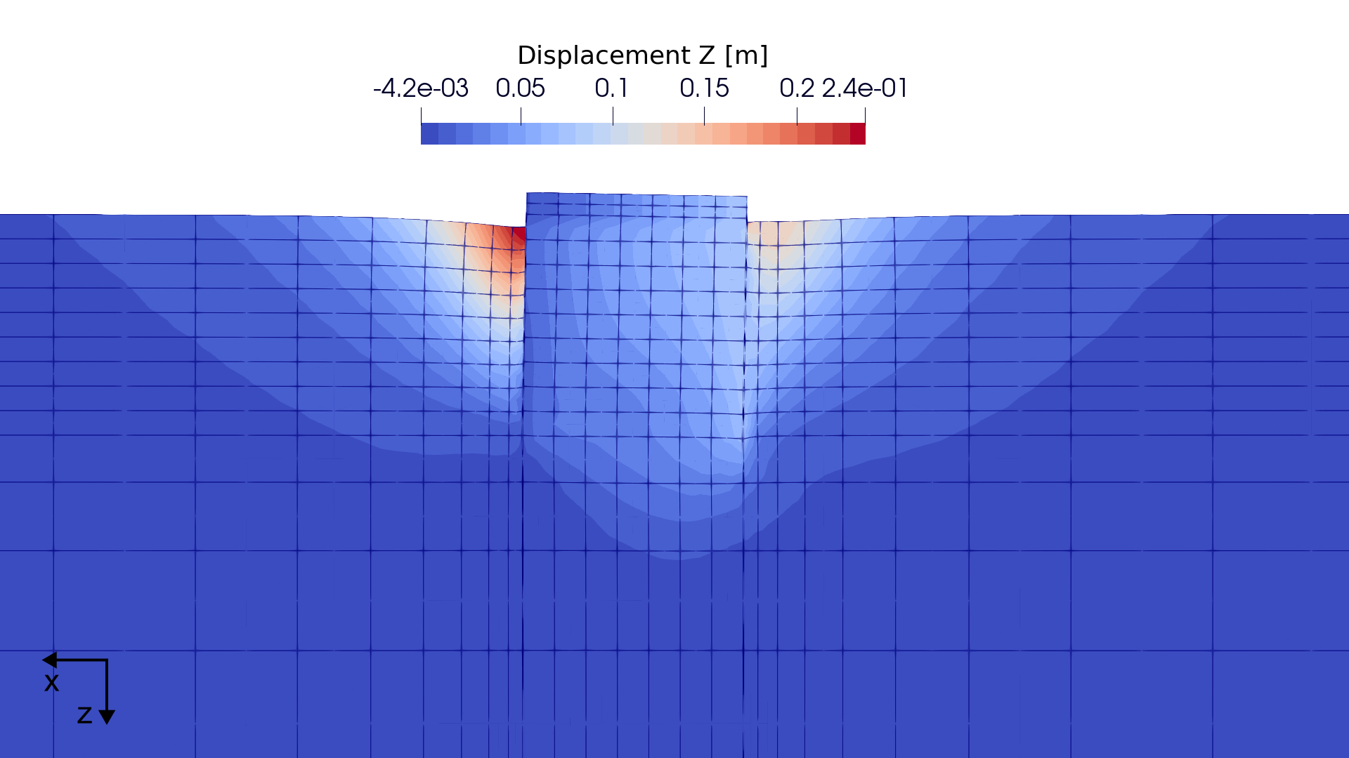 Figure 2. Pattern of vertical displacement at 1 million cycles (5-times enhanced)
The final rotation of the mono caisson about the y-axis, as illustrated in Figure 3, may be created in the form of a diagram in Python.
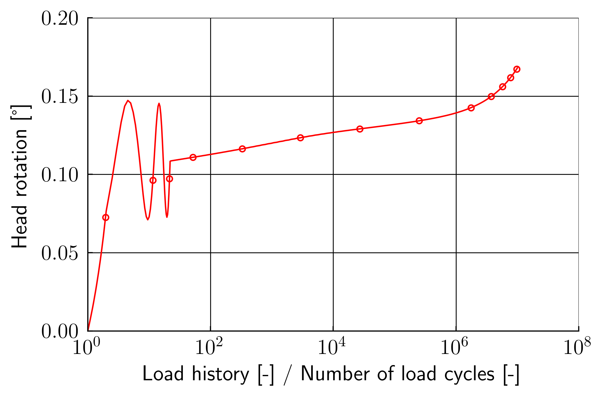 Figure 3. Rotational behavior due to the cyclic loading with number of cycles
-
C. Taylor and P. Hood. A numerical solution of the Navier-Stokes equations using the finite element technique. Computers and Fluids, 1(1):73–100, 1973. URL: https://www.sciencedirect.com/science/article/pii/0045793073900273, doi:10.1016/0045-7930(73)90027-3. ↩
-
T Wichtmann. Soil Behaviour Under Cyclic Loading: Experimental Observations, Constitutive Description and Applications. Habilitation, Institute of Soil Mechanics and Rock Mechanics, Karlsruhe Institute of Technology, Issue No. 181, 2016. ↩