Triaxial Test - Consolidated Drained
Finite Element (FE) representation
For the simulation of consolidated drained (CD) monotonic triaxial tests we perform a so-called ''single-element-simulation'' and by doing so enforce element test assumptions, i.e. a homogeneous distribution of stress/strain within the test sample. A schematic of the FE representation of the CD test is given below.
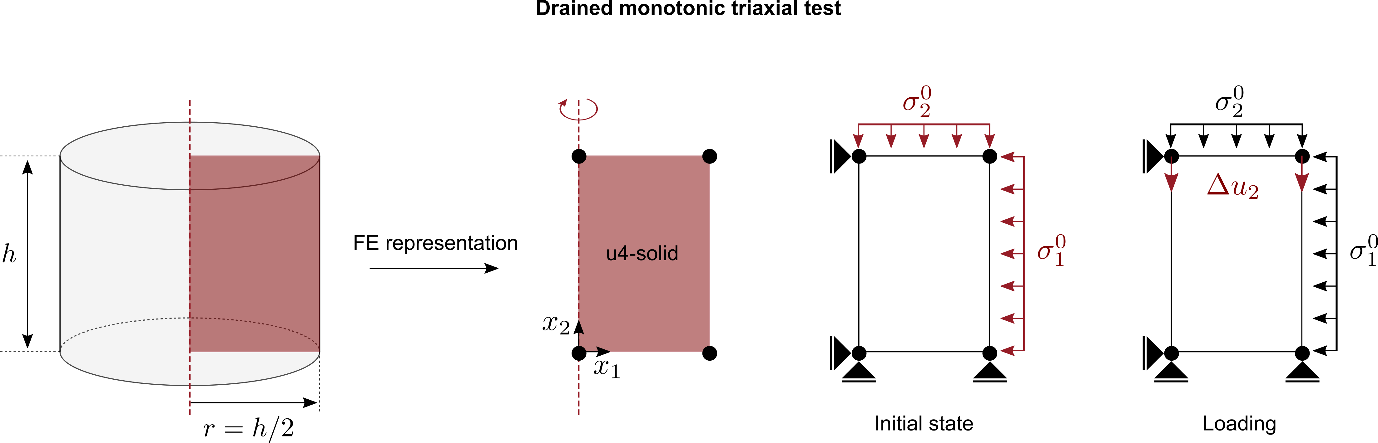
Figure 1. Single-element representation of a drained triaxial compression test
- An axisymmetric solid element with four nodes and linear shape functions for the displacement field is used
- In a first initial step, the initial conditions are applied, i.e. initial stress (\(\sigma_1^0, \sigma_2^0\)), initial void ratio \(e_0\) or any other initial state variable required by the constitutive model to be calibrated
- In the second loading step, the loading is applied by prescribing the vertical displacements \(u_2\) of the top nodes and thus controlling the axial (vertical) strain in the soil. \(u_2\) is increased linearly starting from \(u_2=0\) until \(u_2^{max} = h \cdot \varepsilon_{lab}^{max}\) is reached. Therein, \(h\) is the soil sample and \(\varepsilon_{lab}^{max}\) is the maximum axial strain measured in the laboratory experiment.
Validation of simulation approach
For the validation of the simulation approach, a comparison with the simulation results on Karlsruhe Fine Sand with the Hypo+ISA constitutive model is made.
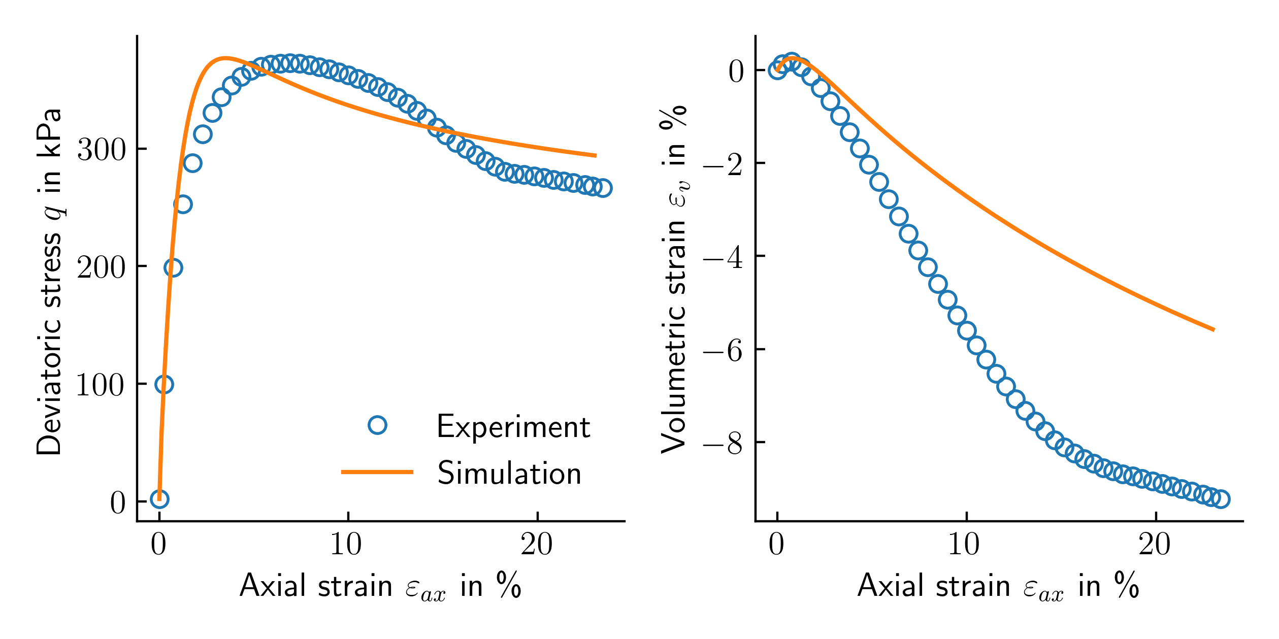
Figure 2. Drained triaxial compression test on Karlsruhe Fine Sand: experiment vs. simulation
Sample numgeo input file
As single-element simulations do not involve complex geometries, we do not use a pre-processor and generate the input file by hand.
-
First we create the four nodes defining the finite element:
*Node 1, 0.0 , 0.00 2, 0.05, 0.00 3, 0.05, 0.1 4, 0.00, 0.10 -
We use an axisymmetric four node solid element (only one phase considered)
*Element, Type = U4-solid-ax 1, 1, 2, 3, 4 -
Next, we define some node and element sets for the assignment of boundary conditions, loads and material parameters:
*Nset, Nset = nall 1, 2, 3, 4 *Nset, Nset = nleft 1, 4 *Nset, Nset = nright 2 , 3 *Nset, Nset = nbottom 1 , 2 *Nset, Nset = ntop 3 , 4 *Elset, Elset=eall 1 -
In order to assign the material to the element, we first create a solid section. The material name linked to this solid section is arbitrary but must be specified in a later step.
*Solid Section, elset = eall, material = soil -
Define the material:
*Material, name = soil, phases = 1 *Mechanical = Hypo-ISA 0.578,9958000.0,0.252,0.643,1.066,1.119,0.155,2.906 1.345,0.000179,0.07,10.149,10.832,0.017,762.0,2.078 *Density 1.8 -
Define the initial conditions of the simulation. In the present case this comprises the definition of the initial (effective) stresses as well as the initial void ratio. The initial stresses will be mandatory in most simulations that you will perform using numgeo. The initial void ratio however is only required for constitutive models incorporating the void ratio as a state variable.
The initial stress is prescribed in terms of the initial effective vertical (or axial) stress \(\sigma_{v0}^\prime\) at two heights of the model and the initial stress ratio \(\sigma_{h0}^\prime/\sigma_{v0}^\prime\) where \(\sigma_{h0}^\prime\) is the horizontal effective stress. In the present example (nearly) isotropic conditions are assumed.
*Initial conditions, type = stress, geostatic
eall, 0.0, -101.58, 0.1, -101.58, 0.981, 0.981
Different constitutive models might require different (internal) state variables to be initialised. For the Hypo+ISA model, initialisation of the void ratio \(e_0\), the intergranular strain tensor \boldsymbol{h}$ and the intergranular back strain tensor \(\boldsymbol{c}\) is required. The intergranular (back) strain is assumed to be isotropically fully mobilised.
*Initial conditions, type = state variables eall, void_ratio, 0.758169085 eall, int_strain11, -0.0001035 eall, int_strain22, -0.0001035 eall, int_strain33, -0.0001035 eall, int_back_strain11, -5.18e-05 eall, int_back_strain22, -5.18e-05 eall, int_back_strain33, -5.18e-05 -
Next, we define an amplitude for later load application. In the present case we use a linear increase from zero at time \(t_{0}=0\) s to one at end time \(t_{end}=1\) s:
*Amplitude, name = LoadingRamp, type = ramp 0.0, 0.0, 1.0, 1.0 -
As in most simulations in geotechnical engineering we start the simulation by initializing the geostatic stress field due to the self weight of the soil and any initial external loading without generating any deformations. In the present case, the initial stress field is solely given by the external load of 500 kPa acting isotropically on the sample. To solve the arising linear system we use a simple lapack solver. Since this is a very basic simulation, we do not request a field output but rely solely on the print output for evaluating the simulation results.
*Step, name=Geostatic, inc=1 *Geostatic *Solver, simple *Body force, instant eall, grav, 0.0, 0., -1, 0. *Dload, instant eall, p3, -101.58 *Dload, instant eall, p2, -99.6 *Boundary nleft, u1, 0. nbottom, u2, 0. *Output, print *Element output, elset=eall S, E, void_ratio *End Step -
In the second step we simulate the shearing of the soil sample by prescribing a linear increasing vertical displacement of the top nodes of the sample. The displacement magnitude at the end of the step is \(u_{end}=0.23\) m which corresponds to an imposed axial strain of \(\varepsilon_{ax}=23\) %.
*Step, name = Loading, inc = 100000, maxiter = 16 *Static 0.005, 1., 0.005, 0.005 *Solver, simple *Body force, instant eall, grav, 0.0, 0., -1, 0. *Dload, instant eall, p3, -101.58 *Dload, instant eall, p2, -99.62 *Boundary, amplitude = LoadingRamp ntop, u2, -0.023 *Boundary nleft, u1, 0. nbottom, u2, 0. *Output, print *Element output, Elset = eall S, E, void_ratio *End Step -
We end the input file by using the "End Step" command.
*End Input
Comparison with experiment
The following Python script was used for the comparison with the experimental data shown in Figure 2. The experimental data can be downloaded here.
#%%
import numpy as np
import matplotlib.pyplot as plt

plt.rcParams['xtick.direction'] = 'in'
plt.rcParams['ytick.direction'] = 'in'
plt.rcParams['text.usetex'] = True
plt.rcParams['font.size'] = 12
plt.rcParams['axes.spines.right'] = False
plt.rcParams['axes.spines.top'] = False

def cm2inch(*tupl):
    inch = 2.54
    if isinstance(tupl[0], tuple):
        return tuple(i/inch for i in tupl[0])
    else:
        return tuple(i/inch for i in tupl)

exp = np.genfromtxt('./KFS-triax-dense.dat', skip_header=2)
sim = np.genfromtxt('./sim-print-out/EALL_element_1.dat', skip_header=1)


fig, (ax1,ax2) = plt.subplots(ncols=2, sharey=False, figsize=cm2inch(16,8))

ax1.plot(exp[::10,0], exp[::10,2], ls='', marker='o', markerfacecolor='None', label='Experiment')
ax1.plot(-sim[:,8]*100, -(sim[:,2]-sim[:,1]), label='Simulation')
ax1.set_ylabel('Deviatoric stress $q$ in kPa')
ax1.set_xlabel('Axial strain $\\varepsilon_{ax}$ in \%')
ax1.legend(loc='lower right', frameon=False)

ax2.plot(exp[::10,0], exp[::10,-1], ls='', marker='o', markerfacecolor='None', label='Experiment')
ax2.plot(-sim[:,8]*100, -(sim[:,7]+sim[:,8]+sim[:,9])*100., label='Simulation')
ax2.set_ylabel('Volumetric strain $\\varepsilon_{v}$ in \%')
ax2.set_xlabel('Axial strain $\\varepsilon_{ax}$ in \%')

fig.tight_layout()

plt.savefig('./triaxCD-exp-vs-sim.png', dpi=400)
plt.show()
Complete input file
The complete input file is given below.
**=~~=~~=~~=~~=~~=~~=~~=~~=~~=~~=~~=~~=~~=~~=~~=~~=~~=~~=~~=~~=~~=~~=~~=~~=~~=
**                                 numgeo-ACT
**                      Copyright (C) 2022 Jan Machacek
**=~~=~~=~~=~~=~~=~~=~~=~~=~~=~~=~~=~~=~~=~~=~~=~~=~~=~~=~~=~~=~~=~~=~~=~~=~~=

*Node
1 , 0.0 , 0.00
2 , 1.0, 0.00
3 , 1.0, 1.0
4 , 0.0, 1.0

*Nset, Nset=nall
1 , 2 , 3 , 4
*Nset, Nset=nleft
1 , 4
*Nset, Nset=nright
2 , 3
*Nset, Nset=nbottom
1 , 2
*Nset, Nset=ntop
3 , 4

*Element, Type=U4-solid-ax
1 , 1 , 2 , 3 , 4

*Elset, Elset = eall
1

** ----------------------------------------

*Solid Section, Elset = eall, material=soil

** ----------------------------------------

*Material, name = soil, phases = 1

*Mechanical = Hypo-ISA
0.578,9958000.0,0.252,0.643,1.066,1.119,0.155,2.906
1.345,0.000179,0.07,10.149,10.832,0.017,762.0,2.078

*Density
1.8

** ----------------------------------------

*Initial conditions, Type = stress, geostatic
eall, 0.0, -101.58, 0.1, -101.58, 0.981, 0.981

*Initial conditions, Type = state variables
eall, void_ratio, 0.758169085
eall, int_strain11, -0.0001035
eall, int_strain22, -0.0001035
eall, int_strain33, -0.0001035
eall, int_back_strain11, -5.18e-05
eall, int_back_strain22, -5.18e-05
eall, int_back_strain33, -5.18e-05

** ----------------------------------------

*Amplitude, name = LoadingRamp, Type=ramp
0.0, 0.0, 1.0, 1.0

** ----------------------------------------

*Step, name=Geostatic, inc=1
*Geostatic

*Solver, simple

*Body force, instant
eall, grav, 0.0, 0., -1, 0.

*Dload, instant
eall, p3, -101.58
*Dload, instant
eall, p2, -99.6

*Boundary
nleft, u1, 0.
nbottom, u2, 0.

*Output, print
*Element output, elset=eall
S, E, void_ratio

*End Step
** ----------------------------------------

*Step, name = Loading, inc = 100000, maxiter = 16
*Static
0.005, 1., 0.005, 0.005
*Solver, simple

*Body force, instant
eall, grav, 0.0, 0., -1, 0.

*Dload, instant
eall, p3, -101.58
*Dload, instant
eall, p2, -99.62

*Boundary, amplitude = LoadingRamp
ntop, u2, -0.23

*Boundary
nleft, u1, 0.
nbottom, u2, 0.

*Output, print
*Element output, Elset = eall
S, E, void_ratio

*End Step

** ----------------------------------------

*End Input