Muskat problem

Validation of element formulations (and implementations) for simulations of partially saturated problems is difficult due to lack of analytical solutions. For this reason, we validate the implementations in numgeo based on a comparison with calculation results obtained with the widely used FE program Plaxis. The boundary value problem (BVP) considered for this purpose is taken from the validation example ''Muskat Problem'' of Plaxis (Vahid Galavi).

The BVP considers the unconfied flow of water in an earth dam. The soil dam has a heigt of 4 m, a width of 1.62 m and is displayed in below figure. The displacements are constrained at all nodes (only the flow of water is investigated in this example). The initial pore water pressure is assumed to be linearly distributed with the water table located at 0.48 m above the bottom boundary. Above 0.48 m the soil is initially partially saturated. During the analysis, the water table on left side of the dam is elevated up to a heigt of 3.22 m above the bottom boundary of the model. The distribution of the phreatic surface in the dam and the height of the seepage face (size saturataed area above the water table on the right-hand side of the dam) are the sought-after variables of this simulation.

Both the soil-water-retention curve and the dependence of the relative permeability on the effective degree of saturation are modelled using the well known van Genuchten model. The hydraulic conductivity $K$ and the parameters of the van Genuchten model are chosen such as described in the Plaxis simulation: $K= 1.7604 \cdot 10^{-6}$ m/s, $n^{vG} = 1.377$ and $\alpha^{vG}=0.383$. The residual degree of saturation is $S^{res}=0.063$. No information about the bulk modulus of the pore water $K^w$ is provided, thus the bulk modulus is assumed to correspond to the one of pure water $K^w = 2.2\cdot 10^6$ kPa. The initial void ratio is $e_0 = 0.5$

Left: finite element model of the BVP, Right: comparison of soil-water-retention curve and relative permeabiltiy used in Plaxis and numgeo.

Input files

The input files for the benchmark simulation can be downloaded here

Material

For the solid a linear elastic constitutive model is chosen. As no soil deformation is considered in this simulation (an neither was observed in the experiment) this choice is completely arbitrary. The Young's modulus is $10^3$ kPa and the Poisson's ratio $0.3$.

Note that numgeo requires the prescription of the permeability $K^s$ of the solid and the dynamic viscosity of the pore fluids $\mu^f$ instead of the hydraulic conductivity $K^f$, which are related as follows: $$ K^f = \dfrac{K^s \gamma^f}{\mu^f} $$

Therein, $\gamma^f$ and $\mu^f$ are the specific weight and the dynamic viscosity of the fluid $f$, respectively.

The dynamic viscosity of pore water is $\mu^w=10^{-6}$ m$\cdot$s and of the pore air $\mu^a=10^{-8}$ m$\cdot$s. Assuming a specific weight of 10 kN/m$^3$ for the pore water, the permeability of the soil is calculated to $1.157407 \cdot 10^{-12}$ m$^2$ (corresponding to 1 m/day).

Geometry and boundary conditions

For the simulation we model the dam as a planar (2D) situation. The dam is discretised with 6-noded triangular elements (quadratic interpolation). The nodal distance is approximately 0.05 m. For this simulation, changes in pore air pressure are judged as negligible, thus elements based on reduced set of governing equations are used - namely the up-formulation. These elements consider negative pore water pressures as suction $s=-p^w$ (instead of $s=p^a-p^w$). The geometry as well as some of the defined node sets are displayed in above figure.

Initial conditions

For the initial pore water pressure the water level is assumed to be located at a height of 0.48 m above the bottom of the model. This results in a linear distribution of pore water pressure taking values of $p^w_0=4.8$ kPa at the bottom, $p^w_0=0$ kPa at 0.48 m and $p^w_0=-35.2$ kPa at the top of the dam. The initial void ratio is $e_0 = 0.5$.

Calculation stages

The simulation is divided into 2 steps in total: - During the Geostatic step, the self weight of the soil (grains and pore water) is applied without generating any deformation. As stated previously, no deformation of the soil skeleton is expected. We therefore constrain the displacements of all nodes in $x1$ and $x2$ direction. In addition, we use boundary conditions to prescribe the pore water pressure for each node. As in the initial conditions, the pore water pressure is prescribed using the hydrostatic option which generates the desired linearly varying distribution. - During the transient step we simulate the water supply at the left side of the dam. This is done by prescribing the pore water pressure at the corresponding nodes using a user defined subroutine. The total step time is 223136 seconds. Due to the strong nonlinearities resulting from the saturation-suction relation and the relative permeability function, we limit the maximum allowed time increment size to 2000 seconds. For the rise of the water level a time of 2.4 hours is assumed.

Results

The following figure presents the comparison of the simulation results obtained with numgeo and the results presented in the validation example of Plaxis by means of the distribution of pore water pressure in steady state conditions. It can be seen, that the pressure distributions obtained by Plaxis and numgeo are in good agreement. Following the phreatic surface (line/surface at which $p^w=0$ kPa holds) the seepage face $s$ can be identified. The calculated seepage face by means of FEM (numgeo and Plaxis) fit reasonably well to the reference analytical solution (Muskat).

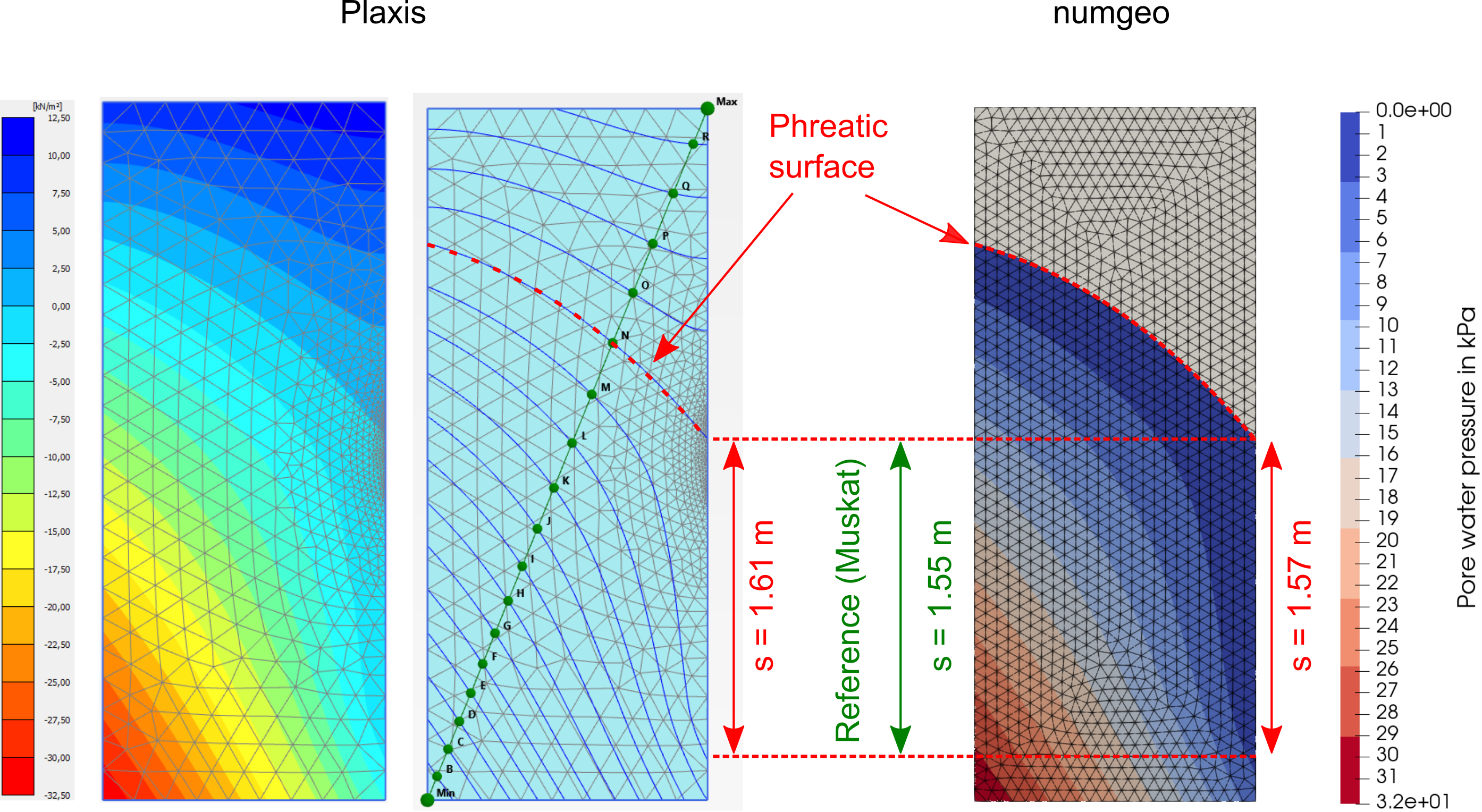Distribution of pore water pressure obtained by Plaxis (left) and numgeo (right) as well as height of the seepage face $s$ (m).