Interaction
*Interaction, Name=<name>, [user]
*Normal,  Mechanical=<>, [no separation], [stiffness_factor=<>], [non constant]
<Normal contact model properties>
*Friction, model=<friction model name>, [stiffness_factor=<>]
<Properties of the friction model>
This keyword is used to define an interaction between two or more individual bodies for contact analyses. The command is followed by one mandatory keyword (Name) and an optional keyword (user):
-
Name=<name>: Set this parameter equal to the name of the interaction (can be chosen freely). This parameter is mandatory. -
The optional
[user]allows for user defined frictional contact properties (in case*Frictionis used) which can vary with respect to coordinates, node label or time. No properties for the frictional contact model have to be defined in the input file in this case, but a user defined file for the contact properties have to given in accordance to the routine described here.
Normal and tangential contact settings
Generally the contact condition can be decomposed into a normal and a tangential (or frictional) behaviour. Note that per default, numgeo assumes frictionless contact. Available models and settings are discussed in the sections Normal contact settings and Tangential contact settings.
Normal contact settings
The *Interaction command must be followed by the definition of the settings of the normal contact using the keyword *Normal. The command is followed by one mandatory keyword (Mechanical) and optional keywords:
-
Mechanical=<>: Set this parameter equal to the mechanical model to describe the normal contact constraint enforcement. The following normal contact models are available:Model Contact tension possible Over-closure relation Penalty no/yes with [no separation] linear -
The optional
[no separation]allows for inseparable contact conditions. Therefore, tension contact conditions are possible. Note that the contact points have to come into contact once before the no separation conditions comes into effect. -
The optional
[stiffness_factor=<>]allows for a user defined stiffness factor used in the evaluation of the penalty factor. The penalty factor is calculated based on the trace of the stiffness matrix of the adjacent continuum element and multiplied with the given stiffness factor. This option only applies if no user defined penalty factor is given (see the following description of the<Normal contact model properties>). The default value of the stiffness factor is 20. -
The optional
[non constant]allows the penalty factor to change during the analysis based on the change of stiffness of the adjacent material. This is beneficial if the material stiffness changes considerably during the analysis, e.g. by spinning-up of a centrifuge. -
The optional
[viscous]allows to consider a normal contact viscosity based on the formula\[ \vec{F}_{\text{Damping}} = -c_n \cdot v_n \cdot \vec{n} \]where:
- \(c_n\): normal damping coefficient
- \(v_n\): normal relative velocity
- \(\vec{n}\): unit normal vector
The damping coefficient can be defined by the user by[viscous]\(=c_n\). The is a second option if the user gives no value. In this case, the coefficient is the normal penalty factor divided by \(10^4\).
The impact of contact viscosity is illustrated below.
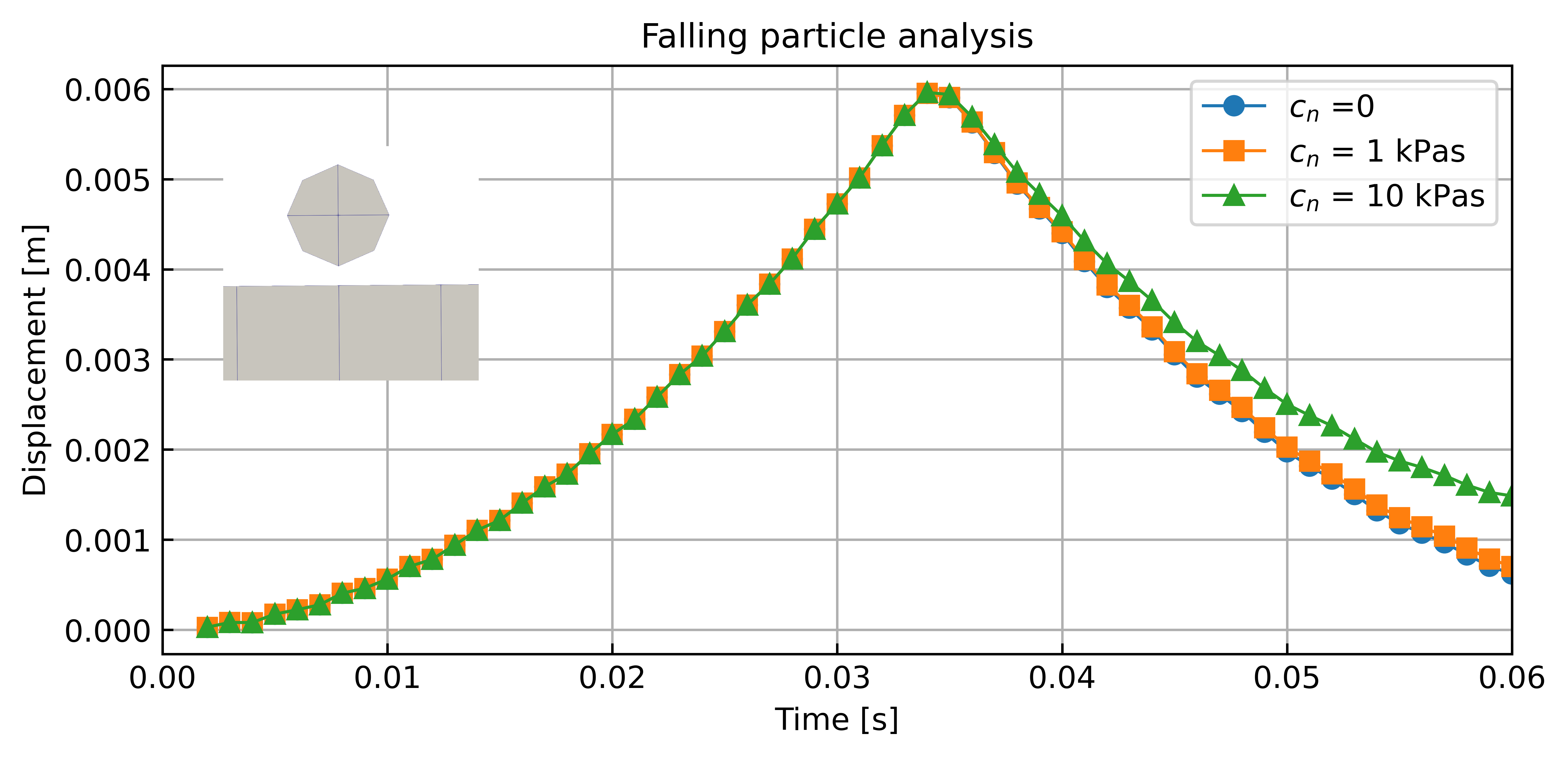
A particle falling by gravity and being reflected when hitting the lower surface for different values of damping coefficients
The *Normal command can be followed by the definition of properties of the normal contact:
-
Normal penalty contact. The following parameter can be defined:
Parameter Unit Mandatory Penalty factor \(\varepsilon\) F/L³ no Adhesion \(c\) F/L² no
- In addition to specifying the (initial) penalty factor, an adhesion acting in the normal direction can also be prescribed. Note that the adhesion is active only if the contact was closed in the previous increment.
Example:
The input lines to define an interaction with name Cont-1 using the Penalty method with a penalty factor of \(10^6\) to enforce the normal contact (no penetration) condition takes the following form:
*Interaction, Name=Cont-1
*Normal, Mechanical = Penalty
1d6
If an adhesion of, for example, 5 kPa is to be prescribed, but nouser defined penalty factor is applied, the contact (no penetration) condition takes the following form:
*Interaction, Name=Cont-1
*Normal, Mechanical = Penalty
,5
Tangential contact settings
In order to activate frictional contact, the *Friction statement must be placed within the scope of the *Interaction definition. The following models for frictional contact are implemented in numgeo:
| Model | Keyword |
|---|---|
| Coulomb friction | Coulomb |
| Coulomb friction | MC , Mohr-Coulomb |
| Hypoplastic friction | Hypoplasticity_numgeo |
Coulomb friction
The keyword for frictional contact following the Coulomb's friction model takes the following form:
*Friction, model=Coulomb, [stiffness_factor=<>]
[ε_T,] tan(δ), c
with the parameters:
| Parameter | Unit | Mandatory | |
|---|---|---|---|
| \(\varepsilon_T\) | Penalty factor tangential | F/A | no |
| \(\tan(\delta)\) | Wall friction angle | - | yes |
| \(c\) | Adhesion | F/A | yes |
Tangential penalty factor
The tangential penalty factor is not mandatory to be given. It is estimated based on the material stiffness if not given (see Section Coulomb friction in the Theory Manual). It is calculated by:
\(G^{mat}\) is being determined automatically by numgeo and is calculated based on the constitutive Jacobian \(\textbf{J}\) of the adjacent element. The scaling factor \(s_T\) has a default value of 1 and can be modified by the user using [stiffness_factor=<>]. In general, it is recommended not to define the \(\varepsilon_T\) directly.
Note on releases before 2026
Before the 2026 release, the Coulomb model was named MC. This was someqhat misleading as dilatation was not considered in the model. With the 2026 release we renamed the model to Coulomb and implemented a proper Mohr-Coulomb type frictional contact model. Note that for backward compatibility reasons, the older keyword model=MC is still valid and interpreted as model=Mohr-Coulomb.
Mohr-Coulomb friction
The keyword for frictional contact following the Mohr-Coulomb's friction model takes the following form:
*Friction, model=Mohr-Coulomb, [stiffness_factor=<>]
[ε_T,] tan(δ), tan(ϑ), c
with the parameters:
| Parameter | Unit | Mandatory | |
|---|---|---|---|
| \(\varepsilon_T\) | Penalty factor tangential | F/A | no |
| \(\tan(\delta)\) | Wall friction angle | - | yes |
| \(\tan(\vartheta)\) | Dilatancy angle | - | yes |
| \(c\) | Adhesion | F/A | yes |
Tangential penalty factor
The tangential penalty factor is not mandatory to be given. It is estimated based on the material stiffness if not given (see Section Coulomb friction in the Theory Manual). It is calculated by:
\(G^{mat}\) is being determined automatically by numgeo and is calculated based on the constitutive Jacobian \(\textbf{J}\) of the adjacent element. The scaling factor \(s_T\) has a default value of 1 and can be modified by the user using [stiffness_factor=<>]. In general, it is recommended not to define the \(\varepsilon_T\) directly.
Hypoplastic friction
The keyword for frictional contact following the hypoplastic friction model as proposed in Staubach et al. (2021)1 takes the following form:
*Friction, model=Hypoplasticity_numgeo
d_s, κ, φ, ν, h_s, n, e_d0, e_c0,
f_ei0, α, β, m_T, m_R, R, β_R, χ
with the parameters:
| Parameter | Unit | |
|---|---|---|
| \(d_s\) | Shear band thickness | Length |
| \(\kappa\) | Surface roughness | - |
| \(\varphi\) | Friction angle | rad |
| \(\nu\) | Poisson's ratio | - |
| \(h_s\) | Granular hardness | F/A |
| \(n\) | Exponent | - |
| \(e_{d0}\) | Minimum void ratio | - |
| \(e_{c0}\) | Maximum void ratio | - |
| \(f_{ei0}\) | Factor \(f_{ei0}\) (\(e_{i0}=f_{ei0}\cdot e_{c0}\)) | - |
| \(\alpha\) | Exponent | - |
| \(\beta\) | Exponent | - |
| \(m_T\) | Intergranular strain multiplier | - |
| \(m_R\) | Intergranular strain multiplier | - |
| \(R\) | Intergranular strain radius | - |
| \(\beta_R\) | Intergranular strain interpolation | - |
| \(\chi\) | Intergranular strain interpolation | - |
Calculations of shear strain
To calculate the shear strain in the interface, specification of a shear band thickness of \(d_s\) in m is required. \(d_s\) is usually assumed to be related to the grain size of the material, e.g. \(d_s \approx 10 d_{10}\). For more information please refer to Staubach et al. (2021)1.
Initial conditions
The hypoplastic interface model requires the initialisation of state variables, namely the void ratio \(e_0\) and the intergranular strain tensor \(\boldsymbol{h}_0\). Further information is provided in the dedicated section Initial contact conditions.
Calcualtion of shear strain
To calculate the shear strain in the interface, specification of a shear band thickness of \(d_s\) in m is required. \(d_s\) is usually assumed to be related to the grain size of the material, e.g. \(d_s \approx 10 d_{10}\). For more information please refer to Staubach et al. (2021)1.
-
Patrick Staubach, Jan Machaček, and Torsten Wichtmann. Novel approach to apply existing constitutive soil models to the modelling of interfaces. International Journal for Numerical and Analytical Methods in Geomechanics, 46(7):1241–1271, may 2022. URL: https://onlinelibrary.wiley.com/doi/10.1002/nag.3344, doi:10.1002/nag.3344. ↩↩↩