Homogeneous slope (Pruška 2009)
Quick read on strength-reduction analysis
The strength reduction method is a separate calculation type that can be selected using the keyword *Reduction in the step definition. During a strength reduction analysis, the shear strength parameters of the soil are incrementally reduced in accordance with a strength reduction factor (SRF) until failure is obtained. The SRF is applied to the tangent of the friction angle and the cohesion to ensure equal proportion of shear resistances by frictional and cohesive terms throughout the strength reduction. Assuming that the factor of safety (FoS) is identical to the SRF, the reduced shear strength parameters \(\varphi_\text{red}\) and \(c_\text{red}\) can be determined based on the actual shear strength parameters and the FoS as follows:
\(\tan \varphi_\text{red} = \tan \varphi\,/\,\text{FoS} \qquad \text{and} \qquad c_\text{red} = c\,/\,\text{FoS}\)
To control the incremental reduction of the shear strength parameters, the line following the keyword *Reduction requires the definition of four scalars: an initial value of the factor of safety (FoS\(_0\)) and an initial step-size (\(\Delta\)FoS\(_0\)), a maximum step-size (\(\Delta\)FoS\(_{\max}\)) and a minimum step-size (\(\Delta\)FoS\(_{\min}\)) need to be prescribed in the calculation type definition. During a strength reduction analysis, FoS is incrementally increased, which results in an incremental reduction of the shear strength parameters.
The strength reduction method can be used in combination with the Mohr-Coulomb and Matsuoka-Nakai model, so far. To specify that the shear strength parameters of a specific material parameter set should be reduced during a strength reduction analysis, the keyword *Reducible Strength needs to be specified in the material definition.
Detection of failure is conducted based on non-convergence. Moreover, post-processing can be used additionally to inspect the maximum displacements vs. FoS. Plotting the former in logarithmic scale, slope failure can also be defined as the FoS associated to a decisive kink in the curve trend.
For the first tutorial on strength reduction we consider a task first presented by Pruška (2009)1 who compared the performance of the geotechnical finite element software products Plaxis, ZSoil and GEO4 (now GEO5). The same example was later used by rocscience to verify the strength-reduction implementation of RS2.
This benchmark features a homogeneous slope with a height of 7 m and a width of 10 m as shown in Figure 1.
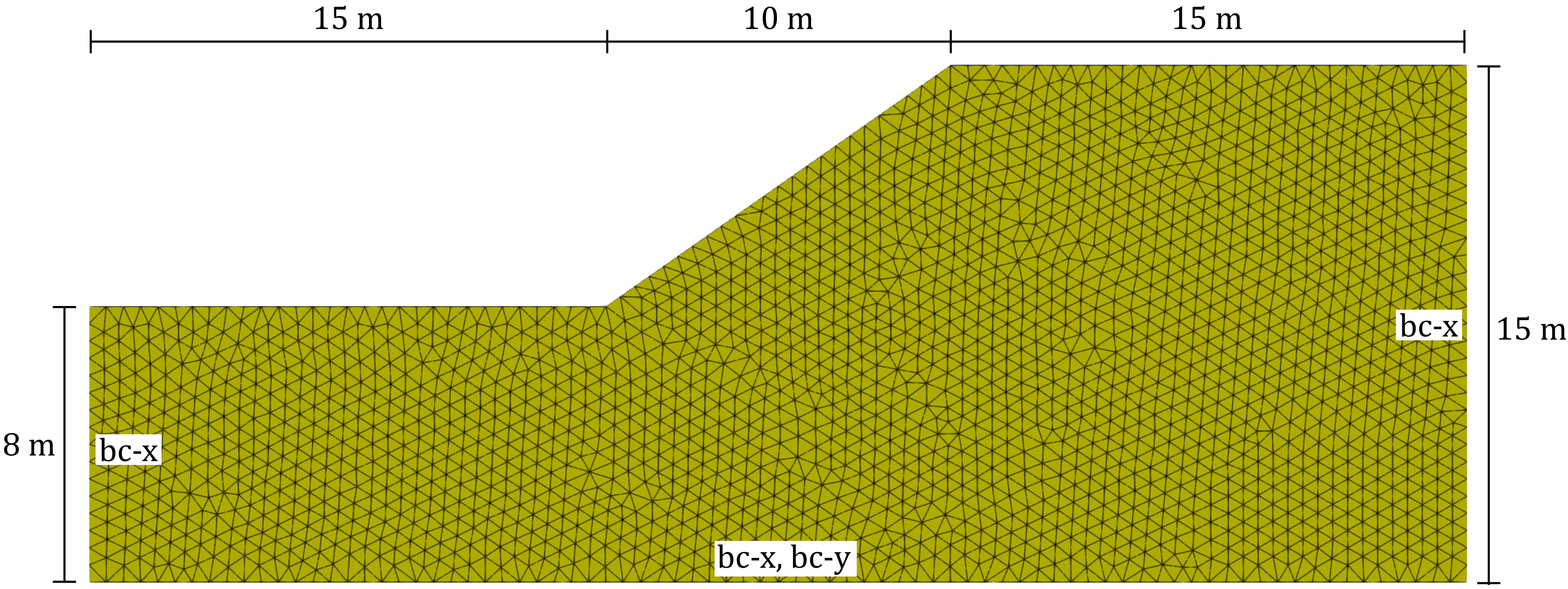
Figure 1. Problem setting and representative finite element mesh of the homogeneous slope used in this tutorial.
Four cases with different soil properties were studied in Pruška (2009)1. The linear elastic, perfectly plastic Mohr-Coulomb (M-C) model was used in the analysis. The material properties of all four cases are as follows:
Table 1. Material parameters for the strength-reduction analyses
| case | \(E\) (kPa) | \(\nu\) | c (kPa) | \(\varphi\) (°) | \(\rho\) (t/m³) |
|---|---|---|---|---|---|
| 1 | 5000 | 0.3 | 20 | 10 | 2.4 |
| 2 | 5000 | 0.3 | 20 | 20 | 2.4 |
| 4 | 5000 | 0.35 | 5 | 20 | 1.8 |
| 5 | 5000 | 0.3 | 20 | 30 | 2.4 |
where \(E\) denotes the Young's modulus, \(\nu\) the Poisson's ratio, \(c\) the effective cohesion and \(\varphi\) the effective friction angle, respectively. \(\rho\) is the density of the soil. The dilatation angle was assumed as \(\psi=0\)° in all cases. No tension cut-off was used. For the back-calculation we will use the Mohr-Coulomb-3 model. Discussion will be limited to case 1 - the other cases can be investigated analogously.
Input files
The input files for the tutorial can be downloaded here and the input files for the cases 2-4 can be downloaded from the corresponding benchmark page.
Finite element mesh
The finite element model was created using the GiD pre-processing software, the corresponding GiD (GUI) files from here. For the discretisation of the domain, two-dimensional u-solid finite elements are used, discretising the displacement (u) of the solid. The mesh is composed of 6-noded triangular elements with quadratic interpolation order (termed u6-solid).
.
.
*Element, Type = U6-solid
.
.
In the mesh file, node sets (NSet) and element sets (ElSet) have been defined to address groups of nodes and elements to be used in the step files (e.g. for the definition of boundary conditions). The following node sets have been defined in the mesh file and used in the step files: bc-x, bc-y, all. Only one element set has been defined: all. For bc-x and bc-y see also Figure 1
To keep the input file as short as possible, we store the finite element mesh in a separate file pruska-2009-mesh.inp and import it at the beginning of the actual input file pruska-2009-case1.inp containing the material and calculation specifications:
*Include = pruska-2003-mesh
Material definition
The material behavior of the soil is described by the Mohr-Coulomb model with material parameters selected as provided in Table 1. We recommend the use of the Mohr-Coulomb-3 implementation. The material model requires the definition of a tension cut-off. Since in this problem statement no tension cut-off is used, we simply prescribe the apex of the Mohr Coulomb criterion as tension cut-off:
\(p_t = \dfrac{c}{\tan \varphi} = 113.4\) kPa
To consider that shear strength parameters of a specific material parameter set should be reduced in a strength reduction analysis, the keyword *Reducible Strength needs to be specified in the material definition.
*Material, name=case1, phases=1
*Mechanical = Mohr-Coulomb-3
5000, 0.3, 20, 10, 0, 113.4
*Density
2.4
*Reducible Strength
Initial conditions
In this example we will start the simulation from a stress-free and gravity-free state and slowly increasing the gravity to establish the initial stress field. Thus no initial state is prescribed.
Amplitudes
Amplitudes need to be defined to allow for changes of loads or boundary conditions during a step. For this example, only a simple loading ramp is needed to incrementally increase the gravity during the first loading step
*Amplitude, Name=loading, Type=ramp
0, 0, 1, 1
Steps
The simulation consists of a total of two steps. During the first step, the gravity is increased starting from 0 m/s² to 10 m/s². In the second step, the strength-reduction is performed to estimate the safety of the system against failure.
Step 1
The gravity increase is performed assuming quasi-static conditions (*Static)
*Step, name=Step 1, inc=1e4, maxiter=32, miniter=1
*Static
0.01, 1, 0.001, 0.1
The displacements of the lateral model boundaries are constrained in horizontal directions, the displacements at the base of the model are constrained in vertical and horizontal direction.
*Solver, Pardiso
*Boundary
bc-x, u1, 0
*Boundary
bc-y, u2, 0
The gravity is increased from its initial value of 0 m/s² to 10 m/s² following a linear relation with the step time:
*Body force, amplitude=loading
all, Grav, 10, 0.0,-1.0,0.0
Finally, we specify the output. In this case, we want to display the simulation results in Paraview. Specifically, we are interested in the displacements u, the stress s and the strain e:
*output, field, VTK, ASCII
*frequency=1
*node output, nset = all
u, s, e,
Lastly we close the step:
*End Step
Step 2
In the second step we perform the strength reduction simulation. With the keyword *Reduction, numgeo uses an automatic procedure to determine the Factor of Safety (FoS) for the current system by incrementally decreasing (and increasing) the shear strength parameters.
*Step, name=Step 2, inc=1e4, maxiter=16, miniter=1
*Reduction
0.9, 0.05, 0.05, 0.0001
The boundary conditions remain unchanged:
*Boundary
bc-x, u1, 0
*Boundary
bc-y, u2, 0
The increase in gravity performed in the first step leads to significant deformations in the system. These are not of relevance for the stability analysis but might render the interpretation of the results more difficult. We thus reset the displacements and strains:
*Reset
Displacement, Strain
The gravity now acts as a constant load
*Body force, instant
all, Grav, 10, 0.0,-1.0,0.0
and we add the Factor of Safety (FoS) to the output request:
*Output, field, VTK, ASCII
*frequency=1
*node output, nset = all
u, S, e,  FoS
Finally, we end the step
*End Step
and close the input file:
*End Input
Results
The displacement contour plot and deformed geometry for case 1 are depicted in Figure 2. The simulation results show a clear failure mechanism resembling a circular slip surface.
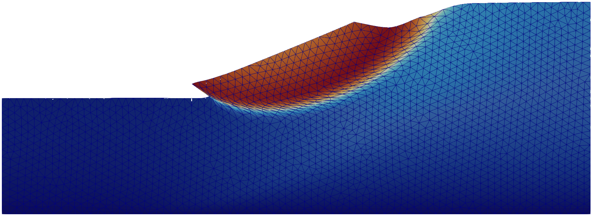
Figure 2. Displacement contour plot and deformed geometry for case 1 calculated with numgeo.
The resulting Factor of Safety (FoS) obtained with numgeo is compared to the results of the four different software packages in Table 2. A very good agreement between the numgeo results and the programs Plaxis, ZSoil and RS2 is attested.
Table 2. Calculated FoS for case 1 for different finite element codes.
| numgeo | Plaxis | ZSoil | GEO4 | RS2 | |
|---|---|---|---|---|---|
| FoS | 1.22 | 1.22 | 1.21 | 1.31 | 1.22 |
Note that the estimation of the slope stability based on non-convergence might yield slight overestimation of the FoS. For this reason, it is emphasized to also inspect the max. displacements vs. FoS plot. In this plot (Figure 3), the critical FoS indicating the level of safety of the slope under investigation can be identified by a sharp kink in the FoS vs. max. displacements or FoS vs. internal energy plots.
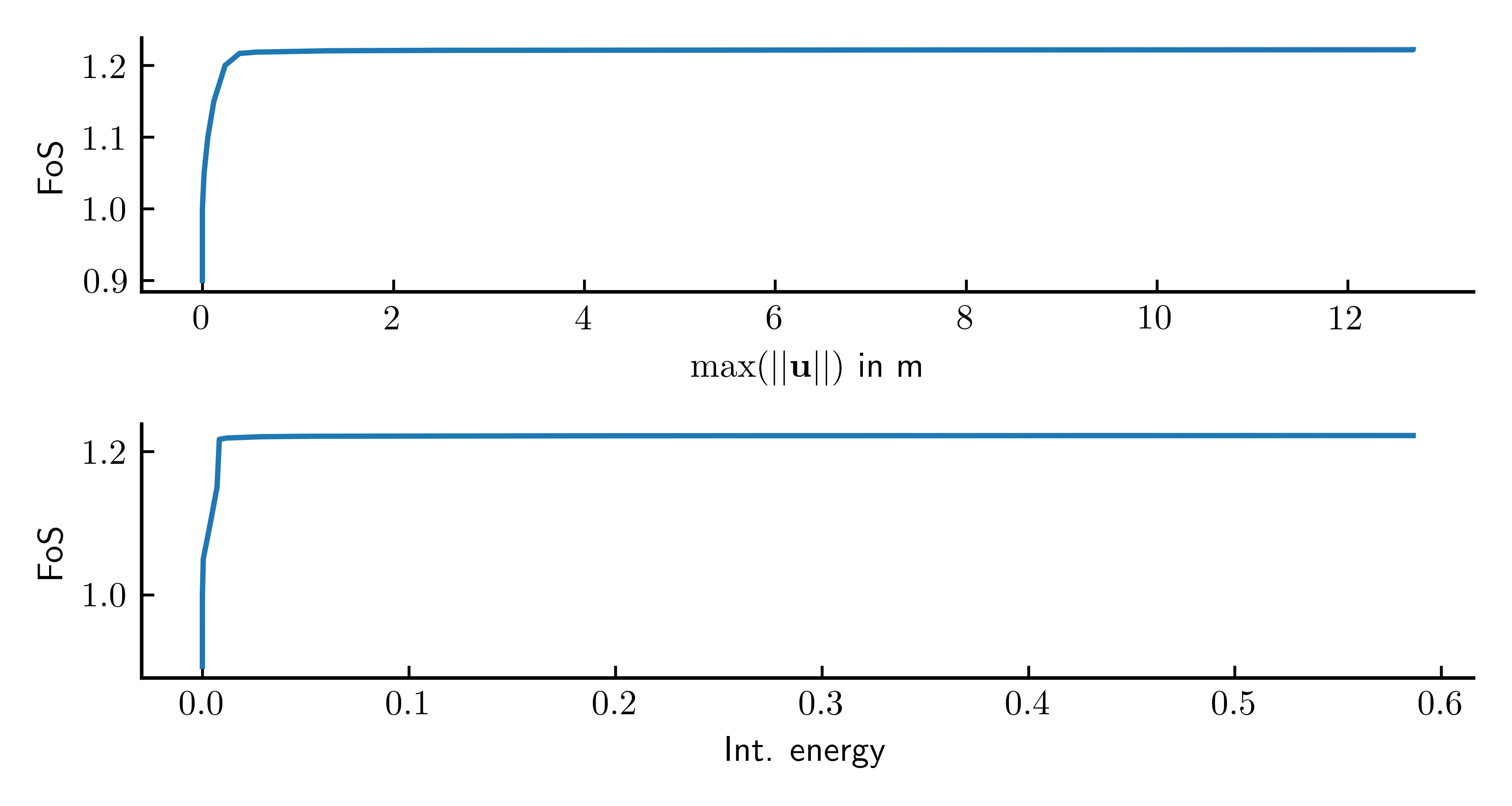
Figure 3. Max. displacement magnitude versus Factor of Safety (FoS) for case 1, calculated with numgeo.
The python script used to produce this plot is given below. The FoS, max. displacement and internal energy data plotted in Figure 3 is saved as an output automatically by numgeo at the end of a strength-reduction analysis and saved in a csv file, here named step2-strength-reduction-history.csv.
#%%
import numpy as np
import matplotlib.pyplot as plt
import pandas as pd

fontsize = 10
plt.rcParams['xtick.direction'] = 'in'
plt.rcParams['ytick.direction'] = 'in'
plt.rcParams['text.usetex'] = True
plt.rcParams['font.size'] = fontsize
plt.rcParams['axes.spines.right'] = False
plt.rcParams['axes.spines.top'] = False
plt.rcParams['axes.linewidth'] = 1.0

# Convert centimeters to inches for figure sizing
def cm2inch(*tupl):
    inch = 2.54
    if isinstance(tupl[0], tuple):
        return tuple(i/inch for i in tupl[0])
    else:
        return tuple(i/inch for i in tupl)


data = np.genfromtxt('./step2-strength-reduction-history.csv', delimiter=',')

fig, ax = plt.subplots(2,1, figsize=cm2inch(15,8), sharex=False)

ax[0].plot(data[:,1],data[:,0])
ax[0].set_xlabel('$\max(||\mathbf{u}||)$ in m')
ax[0].set_ylabel('FoS')
ax[0].set_yticks([0.9,1,1.1,1.2])

ax[1].plot(data[:,2],data[:,0])
ax[1].set_xlabel('Int. energy')
ax[1].set_ylabel('FoS')

plt.tight_layout()

plt.savefig('./pruska-2009-case-fos.png', dpi=600)


fig, ax = plt.subplots(2,1, figsize=cm2inch(15,8), sharex=False)

ax[0].semilogx(data[:,1],data[:,0])
ax[0].set_xlabel('$\max(||\mathbf{u}||)$ in m')
ax[0].set_ylabel('FoS')
ax[0].set_yticks([0.9,1,1.1,1.2])

ax[1].semilogx(data[:,2],data[:,0])
ax[1].set_xlabel('Int. energy')
ax[1].set_ylabel('FoS')

plt.tight_layout()

plt.savefig('./pruska-2009-case-fos-log.png', dpi=600)