Vertical cut slope (Byun 2019)
The second benchmark for strength reduction simulations features a boundary value problem presented by Byun (2019)1 who compared the performance of the geotechnical finite element software products Plaxis, ZSoil and GEO5 and others (no name provided). Amongst other, the stability of a vertical cut slope was analysed using the strength reduction method. The geometry and finite element mesh are shown in Figure 1.
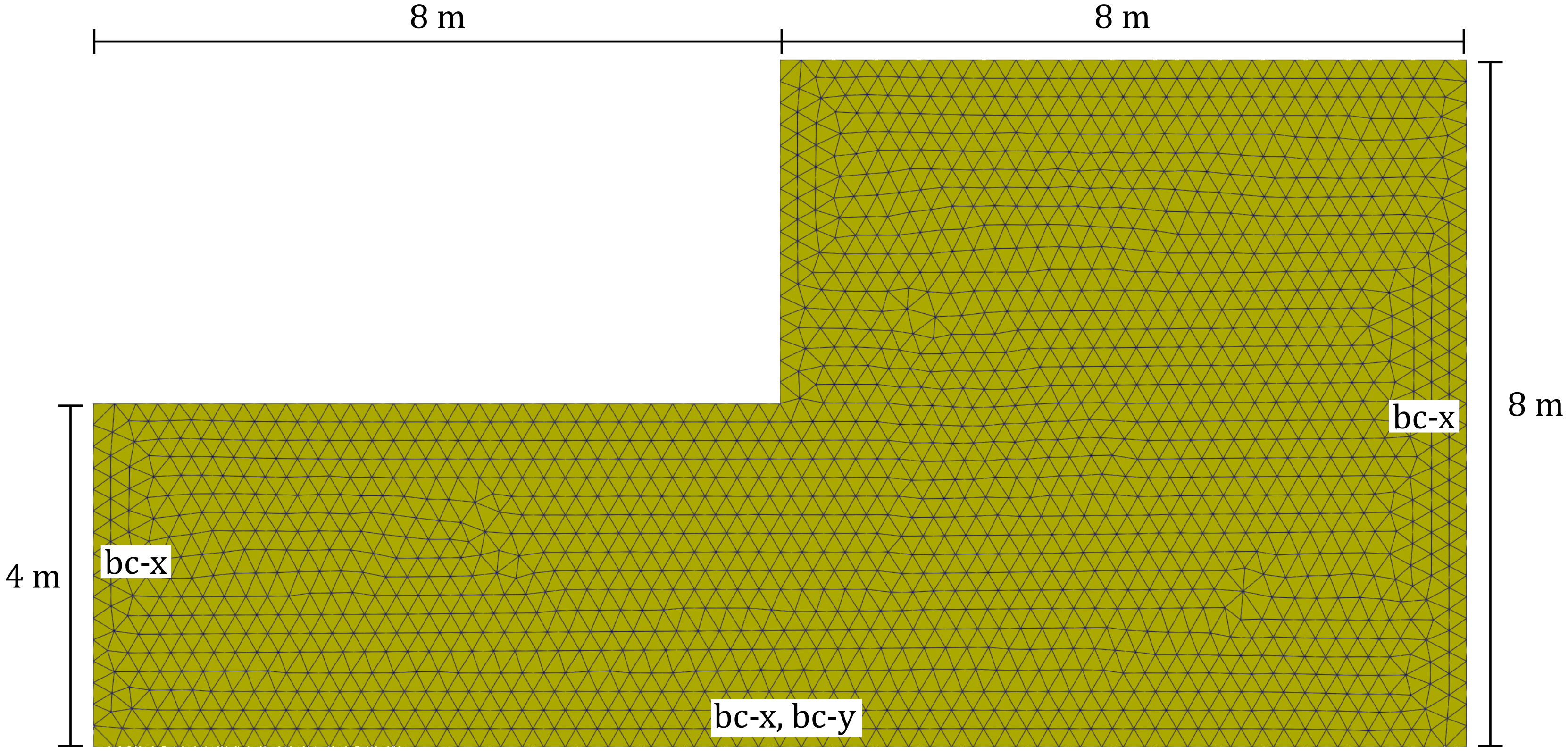
Figure 1. Problem setting and representative finite element mesh of the homogeneous slope used in this tutorial.
The linear elastic, perfectly plastic Mohr-Coulomb model was used in the analysis. The material properties are as follows:
Table 1. Material parameters for the strength-reduction analyses
| \(E\) (kPa) | \(\nu\) | c (kPa) | \(\varphi\) (°) | \(\rho\) (t/m³) |
|---|---|---|---|---|
| 30000 | 0.3 | 16 | 30 | 1.6 |
where \(E\) denotes the Young's modulus, \(\nu\) the Poisson's ratio, \(c\) the effective cohesion and \(\varphi\) the effective friction angle, respectively. \(\rho\) is the density of the soil. The dilatation angle is assumed as \(\psi=0\)°. No tension cut-off is used. For the back-calculation we will use both the Mohr-Coulomb-2 and the Mohr-Coulomb-3 model (one simulation each).
Input files
The input files for the tutorial can be downloaded here. Details on the finite element model and the calculations stages are provided in the corresponding tutorial.
Results
The resulting Factor of Safety (FoS) obtained with numgeo is compared to the results of the five different software packages (and analysis methods) in Figure 2. It can be seen that the results obtained with numgeo are within the range of results obtained with other software and are close to the once obtained with Plaxis.
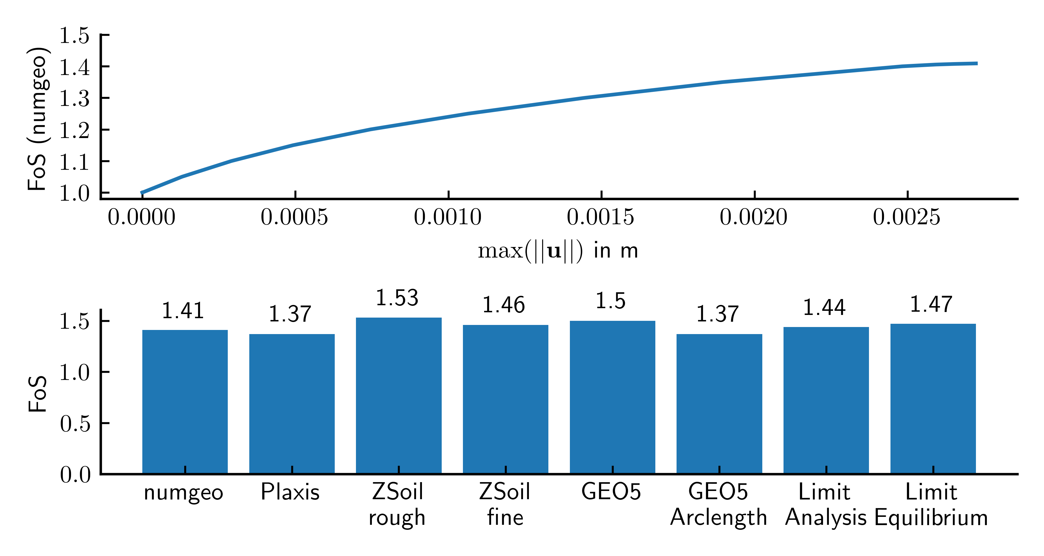
Figure 2. Max. displacement magnitude versus Factor of Safety (FoS) for case 1, calculated with numgeo (top) and comparison to other software (bottom). Two numgeo simulations have been performed, one with the Mohr-Coulomb-2 (elastic jacobian) model and one with the Mohr-Coulomb-3 (elasto-plastic jacobian) model
The python script used to produce this plot is given below.
#%%
import numpy as np
import matplotlib.pyplot as plt

fontsize = 9
plt.rcParams['xtick.direction'] = 'in'
plt.rcParams['ytick.direction'] = 'in'
plt.rcParams['text.usetex'] = False
plt.rcParams['font.size'] = fontsize
plt.rcParams['axes.spines.right'] = False
plt.rcParams['axes.spines.top'] = False
plt.rcParams['axes.linewidth'] = 1.0

# Convert centimeters to inches for figure sizing
def cm2inch(*tupl):
    inch = 2.54
    if isinstance(tupl[0], tuple):
        return tuple(i/inch for i in tupl[0])
    else:
        return tuple(i/inch for i in tupl)


data = np.genfromtxt('./MC2/step3-strength-reduction-history.csv', delimiter=',')
data2 = np.genfromtxt('./MC3/step3-strength-reduction-history.csv', delimiter=',')

fig, ax = plt.subplots(2,1, figsize=cm2inch(16,8), sharex=False)

ax[0].plot(data[:,1]*1000,data[:,0], ls='', marker='o', markerfacecolor=None, label='MC2')
ax[0].plot(data2[:,1]*1000,data2[:,0], label='MC3')
ax[0].set_xlabel('$\max(||\mathbf{u}||)$ in mm')
ax[0].set_ylabel('FoS (numgeo)')
ax[0].set_yticks([1., 1.1, 1.2, 1.3, 1.4, 1.5])
ax[0].legend()

fos = [np.round(data[-1,0],2), np.round(data2[-1,0],2), 1.37, 1.53, 1.46, 1.5, 1.37, 1.44, 1.47]
indices = np.arange(len(fos))
labels = ['numgeo \nMC2', 'numgeo \nMC3','Plaxis', 'ZSoil \nrough', 'ZSoil \nfine', 'GEO5', 'GEO5 \nArclength', 'Limit \nAnalysis', 'Limit \nEquilibrium']

rects = ax[1].bar(labels, fos)
ax[1].bar_label(rects, padding=3)
ax[1].set_ylabel('FoS')
ax[1].set_yticks([0.0, 0.5, 1.0, 1.5])

plt.tight_layout()

plt.savefig('./byun-2019-results-plot.png', dpi=600)
-
G. W. Byun. Comparison between Geotechnical Softwares. In ZSoil Day 2019. 2019-09-25. URL: https://www.zsoil.com/zsoil_day/2019/GW_Byun_Comparision_Geotech_Softwares_2019.pdf. ↩