Contact discretisation

Three different contact discretisation methods are available: the Node-to-Node (NTN), the element-based mortar (EBM) and the segment-based mortar (SBM) method. The latter is only available for 2D analyses.

At the beginning of an analysis with contacts, the Node-to-Node connectivity is evaluated by searching for the closed contact nodes using the euclidean norm. As this search procedure is time consuming, it is done once at the beginning and is repeated only in case the deformations are so large that the connectivity might have changed. This is checked by comparing the total displacement of a contact node with a specific fraction of the length of the element edge to which this node is connected. This fraction is an empirical value and should be large enough to ensure that the nodes are paired correctly. The user is able to modify this fraction in the input file using the option Check Disp of keyword *Contact options (see here). The default value is \(1 ~\%\).

A similar check is made for contact points with a large distance. As they are unlikely to come into active contact, they are not computed in the contact discretisation. This does not only save time, but also avoids problems during evaluation of the contact segments. Again, this is checked by comparing the total displacement of the contact node with a specific fraction of the length of the element edge. The factor used here is considerable larger than the previous one and is by default \(150 ~\%\). The user can modify this factor by using the option Check Dist of keyword *Contact options (see here).

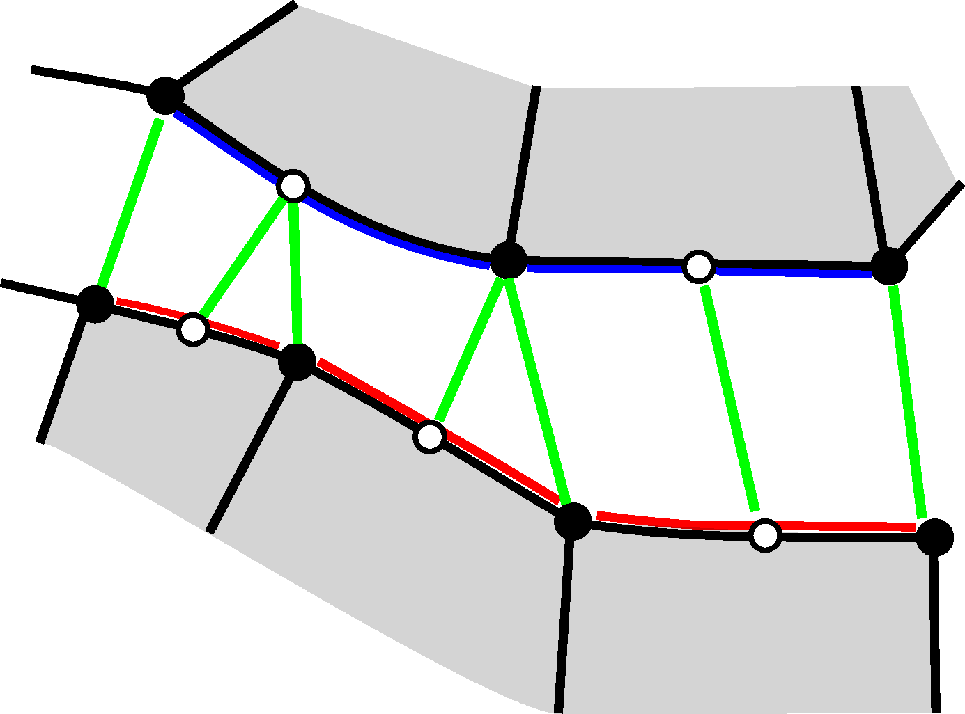
The node-to-node connectivity for a contact pair using quadratically interpolated 2D finite elements is schematically shown in this Figure. Note that the connectivity can change during an analysis due to movement of the two bodies.

Element-based mortar method

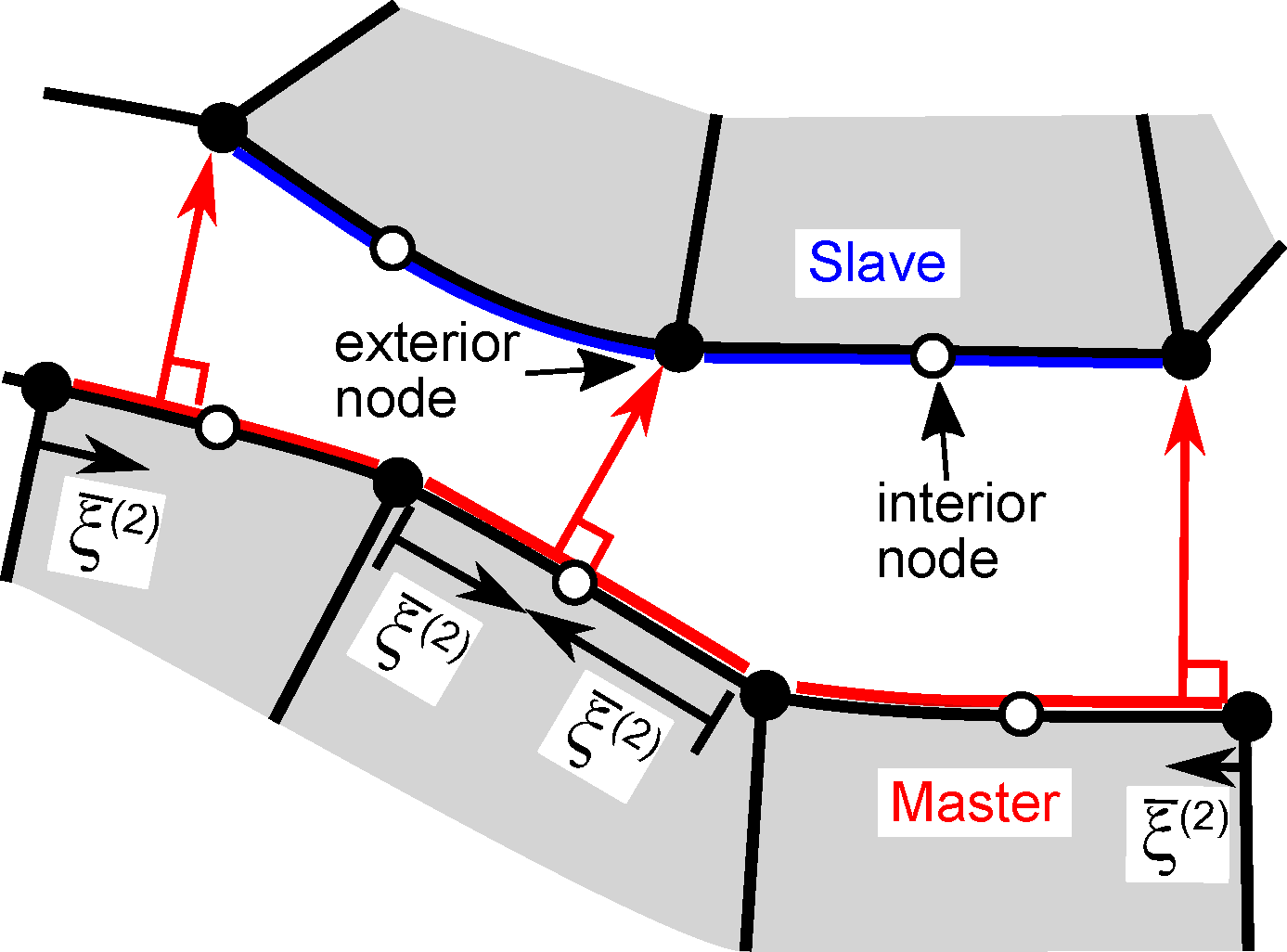
Based on the node-to-node connectivity, the minimum distance between the master and the slave surface is calculated using the convective coordinate \(\bar{\xi}\) (taking values from -1 to 1) along the master surface, which is illustrated in this Figure.

An orthogonal projection of the coordinates \(\boldsymbol{x}_I^{(1)}\) of slave node \(I\) onto the master surface \(\Gamma^{(2)}_c\) is performed for this purpose. This is done by enforcing the tangential vector of the master surface \(\boldsymbol{x}_{,\xi}^{(2)}(\bar{\xi}^{(2)})\) to be orthogonal to the normal gap vector with minimum magnitude between the master surface and slave node \(I\). The projection is defined by

\[ \Big[\sum^{\textrm{nnode}}_J N^{(2)}_J(\bar{\xi}^{(2)})\boldsymbol{x}_J^{(2)}-\boldsymbol{x}_I^{(1)}\Big]\cdot\boldsymbol{x}_{,\xi}^{(2)}(\bar{\xi}^{(2)})= R\stackrel{!}{=} 0, \label{eq_segmentProjection_slave} \]

where the isoparametric description is used to calculate the coordinate of the master surface. To numerically find the solution of Eq. (\(\ref{eq_segmentProjection_slave}\)), Newton's method is applied.

The required derivative of Eq.(\(\ref{eq_segmentProjection_slave}\)) is given by

\[\begin{aligned} K=\frac{\partial R}{\partial \xi}&=\frac{\partial \boldsymbol{g}_{I}(\bar{\xi}^{(2)})}{\partial \xi}\cdot \boldsymbol{x}_{,\xi}^{(2)}(\bar{\xi}^{(2)}) +\boldsymbol{g}_I(\bar{\xi}^{(2)})\cdot \boldsymbol{x}_{,\xi\xi}^{(2)}(\bar{\xi}^{(2)})\nonumber\\ &=\sum^{\textrm{nnode}}_J N_{J,\xi}(\bar{\xi}^{(2)})\boldsymbol{x}_J^{(2)}\cdot \boldsymbol{x}_{,\xi}^{(2)}(\bar{\xi}^{(2)}) + \boldsymbol{g}_I(\bar{\xi}^{(2)})\cdot \boldsymbol{x}_{,\xi\xi}^{(2)}(\bar{\xi}^{(2)}), \end{aligned}\label{eq_dR_dXi}\]

with \(\boldsymbol{g}_I(\bar{\xi}^{(2)})= \Big[\sum^{\textrm{nnode}}_J N^{(2)}_J(\bar{\xi}^{(2)})\boldsymbol{x}_J^{(2)}-\boldsymbol{x}_I^{(1)}\Big]\).

The second term in Eq. (\(\ref{eq_dR_dXi}\)) is only relevant for quadratically interpolated finite elements since \(\boldsymbol{x}_{,\xi\xi}^{(2)}(\bar{\xi}^{(2)})\) is zero otherwise. Note that using quadratically interpolated finite elements, a projection is performed for both exterior (located at the element corner) and interior (located at the element edge/on the element face) nodes (see this Figure).

Determination of the minimum distance between the paired surfaces using the convective coordinate along the master surface (left). Determination of the minimum distance between the paired surfaces using the convective coordinate along the master surface (right).

After Eq. (\(\ref{eq_segmentProjection_slave}\)) is satisfied and \(\bar{\xi}^{(2)}\) obtained, the normal respectively tangential components of the distance of the slave node are calculated by

\[\begin{aligned} g_{N,I}^{(1)} &=\Big[\sum^{\textrm{nnode}}_J N^{(2)}_J(\bar{\xi}^{(2)})\boldsymbol{x}_J^{(2)}-\boldsymbol{x}_I^{(1)}\Big]\cdot\boldsymbol{n}^{(2)} (\bar{\xi}^{(2)})\\ %g^s_N&=(\boldsymbol{x}_{\textrm{igp}}^m-\boldsymbol{x}_{\textrm{igp}}^s)\cdot\boldsymbol{n}_{\textrm{igp}}^s\\ \boldsymbol{g}^{(1)}_{T,I,\alpha}&=\Big[\sum^{\textrm{nnode}}_J N^{(2)}_J(\bar{\xi}^{(2)})\boldsymbol{x}_J^{(2)}-\boldsymbol{x}_I^{(1)}\Big]\cdot\Big[\boldsymbol{\tau}_{\alpha}^{(2)}(\bar{\xi}^{(2)})\otimes\boldsymbol{\tau}_{\alpha}^{(2)}(\bar{\xi}^{(2)})\Big]. %\boldsymbol{g}^s_T&=(\boldsymbol{x}_{\textrm{igp}}^m-\boldsymbol{x}_{\textrm{igp}}^s)\cdot(\boldsymbol{1}-\boldsymbol{n}_{\textrm{igp}}^s\otimes\boldsymbol{n}_{\textrm{igp}}^s) \end{aligned}\label{eq_tang_gap_STS}\]

\(\boldsymbol{n}^{(2)} (\bar{\xi}^{(2)})\) is the normal vector of the master surface at the local coordinate \(\bar{\xi}^{(2)}\) and is defined here. \(\boldsymbol{\tau}_{\alpha}^{(2)}(\bar{\xi}^{(2)})\) is the tangential vector in direction \(\alpha=1,2\) (if the problem is three-dimensional) introduced here.

For frictional problems, the increment of the tangential gap \(\Delta \boldsymbol{g}_{T,\alpha}\) is required. It is calculated by

\[\begin{aligned} \Delta \boldsymbol{g}^{(1)}_{T,I,\alpha}&=\Big[\sum^{\textrm{nnode}}_J N^{(2)}_J(\bar{\xi}^{(2)})\Delta\boldsymbol{u}_J^{(2)}-\Delta \boldsymbol{u}_I^{(1)}\Big]\cdot\Big[\boldsymbol{\tau}_{\alpha}^{(2)}(\bar{\xi}^{(2)})\otimes\boldsymbol{\tau}_{\alpha}^{(2)}(\bar{\xi}^{(2)})\Big]. \end{aligned}\label{eq_tang_gap2_STS}\]

\(g_{N,I}\) and \(\boldsymbol{g}_{T,I,\alpha}\) defined in Eq. (\(\ref{eq_tang_gap_STS}\)) determine the contact distance for node \(I\) of the slave surface. In order to determine the respective values for the master node \(J\), the convective coordinate \(\bar{\xi}^{(1)}\) along the slave surface is computed, viz.

\[\begin{aligned} \Big[\sum^{\textrm{nnode}}_I N^{(1)}_I(\bar{\xi}^{(1)})\boldsymbol{x}_I^{(1)}-\boldsymbol{x}_J^{(2)}\Big]\cdot\boldsymbol{x}_{,\xi}^{(1)}(\bar{\xi}^{(1)})= 0. \end{aligned}\label{eq_conv_coord_STS_slave}\]

The normal and tangential distances given by Eq. ((\(\ref{eq_tang_gap_STS}\)) are then evaluated using \(\bar{\xi}^{(1)}\) to obtain \(g^{(2)}_{N,J}\) and \(\boldsymbol{g}^{(2)}_{T,J}\), defining the normal and tangential gap of the master node \(J\).

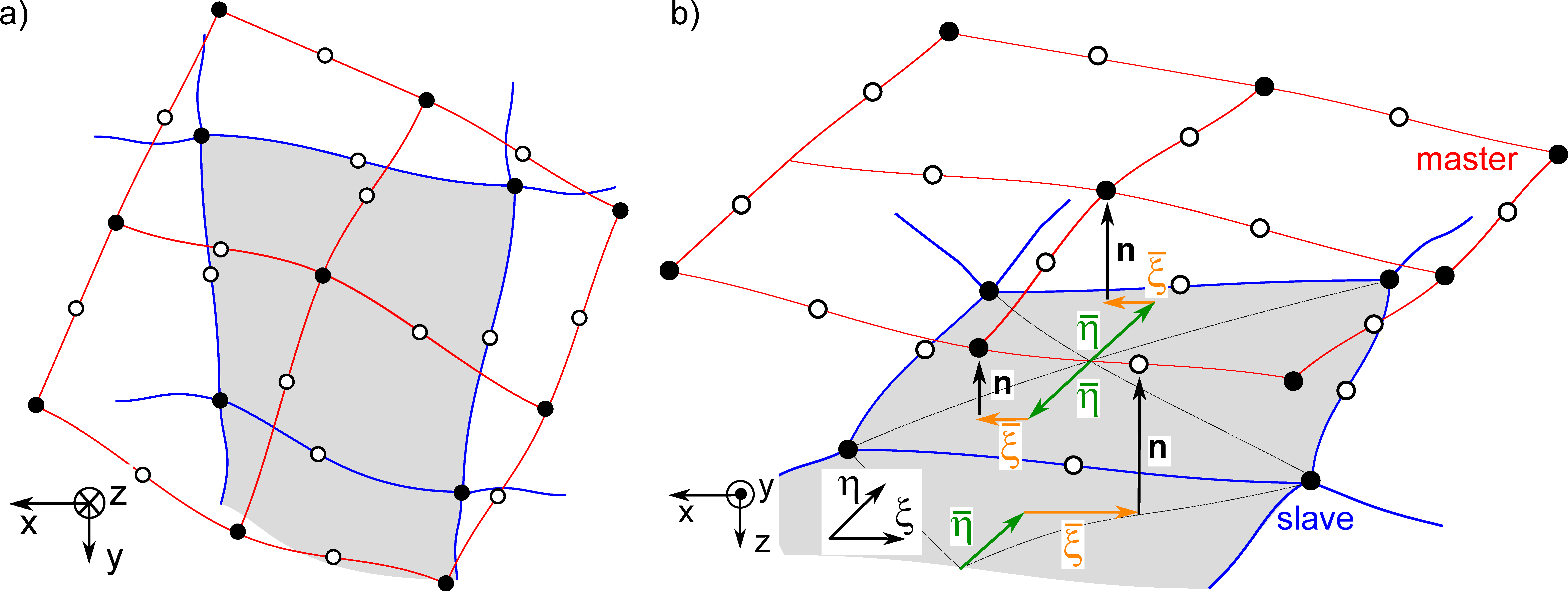
For three-dimensional analyses, the convective coordinate has two components since the projection is performed on a face rather than a line. For the projection of the location of the slave node onto the face of the master surface, the convective coordinates \(\bar{\xi}^{(2)}\) and \(\bar{\eta}^{(2)}\) are evaluated by

\[\begin{aligned} \Big[\sum^{\textrm{nnode}}_J N^{(2)}_J(\bar{\xi}^{(2)},\bar{\eta}^{(2)})\boldsymbol{x}_J^{(2)}-\boldsymbol{x}_{I}^{(1)}\Big]\cdot\boldsymbol{x}_{,\xi}^{(2)}(\bar{\xi}^{(2)},\bar{\eta}^{(2)})&= 0\\ \Big[\sum^{\textrm{nnode}}_J N^{(2)}_J(\bar{\xi}^{(2)},\bar{\eta}^{(2)})\boldsymbol{x}_J^{(2)}-\boldsymbol{x}_{I}^{(1)}\Big]\cdot\boldsymbol{x}_{,\eta}^{(2)}(\bar{\xi}^{(2)},\bar{\eta}^{(2)})&= 0. \end{aligned}\label{eq_Nts_projection3d_eta}\]

Eqs. (\(\ref{eq_Nts_projection3d_eta}\)) are solved simultaneously using Newton's method. The required derivatives of Eqs. (\(\ref{eq_Nts_projection3d_eta}\)) build a two times two matrix in this case. The local convective coordinates are updated every \(n\)-th iteration by

\[\begin{aligned} \left[\begin{array}{l} \bar{\xi}^{(2)}\\ \bar{\eta}^{(2)}\\ \end{array}\right]_{n+1} = &\left[\begin{array}{l} \bar{\xi}^{(2)}\\ \bar{\eta}^{(2)}\\ \end{array}\right]_{n} - \left[\begin{array}{ll} \boldsymbol{g}_I(\bar{\xi}^{(2)},\bar{\eta}^{(2)})\cdot\boldsymbol{x}_{,\xi}^{(2)}(\bar{\xi}^{(2)},\bar{\eta}^{(2)})& \boldsymbol{g}_I(\bar{\xi}^{(2)},\bar{\eta}^{(2)})\cdot\boldsymbol{x}_{,\eta}^{(2)}(\bar{\xi}^{(2)},\bar{\eta}^{(2)})\\ \end{array}\right]_{n}\nonumber\\ &\cdot\left[\begin{array}{ll} \dfrac{\partial}{\partial \bar{\xi}^{(2)}}\Big[ \boldsymbol{g}_I(\bar{\xi}^{(2)},\bar{\eta}^{(2)})\cdot\boldsymbol{x}_{,\xi}^{(2)}(\bar{\xi}^{(2)},\bar{\eta}^{(2)})\Big]& \dfrac{\partial}{\partial \bar{\xi}^{(2)}}\Big[ \boldsymbol{g}_I(\bar{\xi}^{(2)},\bar{\eta}^{(2)})\cdot\boldsymbol{x}_{,\eta}^{(2)}(\bar{\xi}^{(2)},\bar{\eta}^{(2)})\Big]\\ \dfrac{\partial}{\partial \bar{\eta}^{(2)}}\Big[ \boldsymbol{g}_I(\bar{\xi}^{(2)},\bar{\eta}^{(2)})\cdot\boldsymbol{x}_{,\xi}^{(2)}(\bar{\xi}^{(2)},\bar{\eta}^{(2)})\Big]& \dfrac{\partial}{\partial \bar{\eta}^{(2)}}\Big[ \boldsymbol{g}_I(\bar{\xi}^{(2)},\bar{\eta}^{(2)})\cdot\boldsymbol{x}_{,\eta}^{(2)}(\bar{\xi}^{(2)},\bar{\eta}^{(2)})\Big]\\ \end{array}\right]_{n}^{-1}. \end{aligned}\]

In analogy to the EBM method for 2D analyses, the projection is also performed on the faces of the finite elements of the slave surface to evaluate the minimum distances of the master node. Hence, the equations

\[\begin{aligned} \Big[\sum^{\textrm{nnode}}_I N^{(1)}_I(\bar{\xi}^{(1)},\bar{\eta}^{(1)})\boldsymbol{x}_I^{(1)}-\boldsymbol{x}_{J}^{(2)}\Big]\cdot\boldsymbol{x}_{,\xi}^{(1)}(\bar{\xi}^{(2)},\bar{\eta}^{(2)})&= 0\\ \Big[\sum^{\textrm{nnode}}_I N^{(1)}_I(\bar{\xi}^{(1)},\bar{\eta}^{(1)})\boldsymbol{x}_I^{(1)}-\boldsymbol{x}_{J}^{(2)}\Big]\cdot\boldsymbol{x}_{,\eta}^{(1)}(\bar{\xi}^{(2)},\bar{\eta}^{(2)})&=0 \end{aligned}\label{eq_Nts_projection3d_eta_slave}\]

are iteratively solved.

The evaluation of the convective coordinates for 3D analyses is schematically shown in this Figure. The grey element face indicates the slave surface for which the local convective coordinates are evaluated solving Eqs. (\(\ref{eq_Nts_projection3d_eta_slave}\)) simultaneously using Newton's method. The convective coordinates are exemplary evaluated for 3 nodes of the master surface.

During the minimisation of Eqs. (\(\ref{eq_Nts_projection3d_eta_slave}\)) the local coordinates may exceed the boundaries of the element (\(\{\|\bar{\xi}\|,\|\bar{\eta}\|\}> 1\)). In this case, the minimisation has to continue with the face of the next element to which the local coordinates point. Different cases have to be distinguished when evaluating the element face for which the projection continues depending on the value of the local coordinates and the local node label of the current element. If the convective coordinates reach a \"natural\" border, i.e. the coordinates are spatially outside the defined surface zone, the mechanism stops.

Evaluation of the convective coordinates of the slave surface for 3D analyses. Figure a) shows the top-view on the surfaces. The exemplary evaluation of the convective coordinates of the slave surface by projection to three master nodes is given in Fig. b).

The normal contact distance and increment in relative tangential movement are determined at the surface nodes. For the integration of the resulting contact stress, an interpolation to the integration points of the surface is made. The integration of surface loads is performed analogously to the integration of finite elements. Alternatively, the evaluation of the convective coordinates may be directly done for the coordinates of the integration points of the surface. \(\boldsymbol{x}_{I}^{(1)}\) in Eqs. (\(\ref{eq_Nts_projection3d_eta}\)) and \(\boldsymbol{x}_{J}^{(2)}\) in Eqs. (\(\ref{eq_Nts_projection3d_eta_slave}\)) are replaced by \(\sum^{\textrm{nnode}}_I N^{(1)}_I(\xi^{(1)}_\textrm{igp},\eta^{(1)}_\textrm{igp})\boldsymbol{x}_{I}^{(1)}\) and \(\sum^{\textrm{nnode}}_J N^{(2)}_J(\xi^{(2)}_\textrm{igp},\eta^{(2)}_\textrm{igp})\boldsymbol{x}_{J}^{(2)}\) in this case. An interpolation of the contact variables is not necessary using this approach. Both techniques are implemented in numgeo. By default, the latter approach is used. However, if water contact is active or a numerical differentiation is used to evaluate the contributions of the contact constraints to the left-hand side, the node based scheme is used.

The implemented EBM method allows adding additional nodes or integration points to the surface. This is beneficial, since the contact stress is in general non-constant with respect to the surface geometry. Its determination and integration is thus more precise if more discrete points on the surface are considered. For this, artificial nodes/integration points are generated at the surface, which are located at the local coordinates of the underlying finite elements at which integration points would exist if finite elements with higher order would be used. Hence, the surface operations are performed as if finite elements with a higher order of interpolation are used, but the drawback of higher computational effort in computation of the continuum using a larger number of discrete points is circumvented.

The EBM method is implemented in combination with the penalty regularisation introduced in Section [subsec_penalty]{reference-type="ref" reference="subsec_penalty"}. The normal contact contribution to the force equilibrium using the EBM discretisation technique is given by

\[\begin{aligned} \boldsymbol{r}_{N,I}^{(i)}= \sum_{\textrm{igp}}^{\textrm{ngp}}N^{(i)}_I(\xi^{(i)}_{\textrm{igp}}) t^{(i)}_{N,\textrm{igp}} \boldsymbol{n}_{\textrm{igp}}^{(i)} w^{(i)}_{\textrm{igp}} j^{(i)}_{\textrm{igp}} ~~ \textrm {for}~~ i=\{1,2\}, \end{aligned}\label{eq_rhs_STS_main}\]

if the contact stress is directly evaluated at the integration points of the finite-element edge or face. The normal contact stress \(t^{(i)}_{N,\textrm{igp}}\) is calculated by multiplying the normal distance with the penalty factor.

For three-dimensional analyses, the contribution to the force equilibrium of the frictional contact forces \(\boldsymbol{r}_{T,I}^{(i)}\) is calculated using

\[\begin{aligned} %\boldsymbol{r}^{(i),~\textrm{mortar}}_{T,I}= %\sum_{\textrm{igp}}^{\textrm{ngp}}N^{(i)}_I[\xi(\eta_{\textrm{igp}})] t^{(i)}_{T,\textrm{igp},j} \boldsymbol{\tau}^{(i)}_{\textrm{igp},j} w^{(i)}_{\textrm{igp}} j^{(i)}_{\textrm{igp}} ~~ \textrm {for}~~ i,j=\{1,2\}\mand \boldsymbol{r}^{(i)}_{T,I}= \sum_{\alpha}^{\textrm{ndim-1}}\sum_{\textrm{igp}}^{\textrm{ngp}}N^{(i)}_I(\xi^{(i)}_{\textrm{igp}}) t^{(i)}_{T,\textrm{igp},\alpha} \boldsymbol{\tau}^{(i)}_{\textrm{igp},\alpha} w^{(i)}_{\textrm{igp}} j^{(i)}_{\textrm{igp}} ~~ \textrm {for}~~ i=\{1,2\}. \end{aligned} \label{eq_rhs_friction_LHS_main}\]

The required derivatives of Eqs. (\(\ref{eq_rhs_STS_main}\), \(\ref{eq_rhs_friction_LHS_main}\)) with respect to the primary variables for the LHS can be found in ¹.

Segment-based mortar method

Details on the implementation may be found in ².

Contact iterations

Due to the added non-linearities, contact analyses may need special treatment of the constraints in order to achieve good convergence rates if two bodies come into contact driven by Neumann boundary conditions and one of the bodies is not constrained by any Dirichlet boundary condition (e.g. a pile driven by force into soil). If contacts open or close, entries in RHS and LHS with large values are removed or added, respectively. This causes jumps in the solution, causing the global Newton-Raphson iteration to fail to converge. Special contact iterations are introduced for such cases. During a contact iteration, the contact contributions to the global system of equations are iteratively refined until no nodes change their contact status and the change in contact stress from one contact iteration to the next is below a tolerance. As long as these two requirements are not met, the updated contact contributions are only added to the slave and not to the master surface. Note that if a previous iteration involved a contact iteration, at least two additional iterations with consideration of the contact contributions to RHS and LHS of the master surfaces are required, i.e. the iteration is not finished in case of convergence if the contact contributions to the master surface are considered for the first time. Otherwise, the displacement of the master body following the first update of the contact contributions is only taken into account with the correction \(\mathbf{c}^{(i)}\) and no subsequent call of the contact algorithms is made.

Integration of contact contributions using serendipity elements

Following the Taylor-Hood formulation ³, the solid displacement of the hydro-mechanically coupled finite element formulations (u-p or u-p-U) is conventionally interpolated using quadratic interpolation functions. The fluid pressure is interpolated using linear interpolation functions. Otherwise, the LBB condition is not fulfilled and numerical stability not secured. For 3D elements, the interpolation functions using 20 nodes are usually applied for the interpolation of the displacement. This so-called serendipity element does not use the standard Lagrangian bi/tri-quadratic interpolation functions.

The integration of the shape functions used for quadratically interpolated serendipity elements can lead to a negative area/volume, which is not physical ⁴⁵. This is problematic in contact analyses, as the convergence rate is heavily influenced by this error in the integration of the contact stress and contributions to LHS on the element faces ⁶. However, the primarily used element type in geotechnical analysis with pore fluid pressure DOF is the quadratically interpolated serendipity element.

A solution for the problem of surface integration of 3D serendipity elements in contact analyses has been proposed by ⁴, adding an additional node to the face of the serendipity element being in contact. Note that both the shape functions used for the integration of the face as well as the shape functions of the finite element have to be modified. It is not sufficient to only integrate the surface with an additional node, which has been tested in the course of this work. The approach by ⁴ requires a distinction during assembly of RHS and LHS, since finite elements with contact contributions have to be interpolated and integrated differently than regular finite elements. From a programming point of view this is not ideal. Therefore, a transformation of any serendipity element to a full tri-quadratically interpolated element using standard Lagrangian shape functions in case of 3D contact analyses is implemented. This element has 27 nodes and does not suffer from the aforementioned problems in contact analyses.

Since some pre-processors do not allow for the generation of 27-node brick elements (referred to as u27 element), the generation of the additional nodes required for the transformation of the 20-node brick element (u20) to the 27-node element is implemented in numgeo. The additional nodes are also added automatically to existing node-set definitions.

To show the differences in terms of convergence rate between the u20 and u27 element, the change in the norm of residual energy (for definition see ⁷) with respect to the number of iterations for a contact analysis with two elastic bodies coming in initial contact is given in this Figure (a penalty factor of \(\varepsilon = 100\cdot E\) is used to enforce the non-penetration condition, where \(E\) is Young's modulus). The u27 element converges in one iteration yielding perfect equilibrium. The convergence rate of the u20 element is considerably worse.

A major drawback of the u27 elements, compared to the u20 elements, is that a reduced numerical integration is not possible. The u20 elements allow for an integration using 8 integration points instead of a "full" integration with 27 points without showing communicable hourglass modes. Contrary to that, u27 elements show strong hourglassing for 8, 14 or 15 integration points (for the integration rules see ⁸). All three integration rules have been tested and are found to be not feasible. To the author's best knowledge, no hourglass-stiffness enhanced reduced integrated u27 element formulation is reported in the literature.

Change of the norm of residual energy with respect to number of iteration for the simulation of two elastic bodies coming into contact for the `u20` and `u27` element, respectively

Note that the trouble of surface integration of serendipity elements exists only for 3D analyses. The integration of the element edge of 2D serendipity elements does not show the aforementioned errors since standard Lagrangian interpolation functions are used for the 1D edges.

---

1. P. Staubach. Contributions to the numerical modelling of pile installation processes and high-cyclic loading of soils. 2022. doi:10.13154/294-9088. ↩

2. Patrick Staubach, Jan Machaček, and Torsten Wichtmann. Mortar contact discretisation methods incorporating interface models based on Hypoplasticity and Sanisand: Application to vibratory pile driving. Computers and Geotechnics, 146:104677, jun 2022. URL: https://www.sciencedirect.com/science/article/pii/S0266352X2200043X https://linkinghub.elsevier.com/retrieve/pii/S0266352X2200043X, doi:10.1016/j.compgeo.2022.104677. ↩

3. C. Taylor and P. Hood. A numerical solution of the Navier-Stokes equations using the finite element technique. Computers and Fluids, 1(1):73–100, 1973. URL: https://www.sciencedirect.com/science/article/pii/0045793073900273, doi:10.1016/0045-7930(73)90027-3. ↩

4. R Buczkowski. 21-node hexahedral isoparametric element for analysis of contact problems. Communications in Numerical Methods in Engineering, 14:681–692, 1998. doi:10.1002/(SICI)1099-0887(199807)14:7<681::AID-CNM182>3.0.CO;2-T. ↩↩↩

5. Robert D Cook, David S Malkus, Michael E Plesha, and Robert J Witt. Concepts and Applications of Finite Element Analysis. John Wiley & Sons, 2007. ISBN 0470088214. ↩

6. Kent T. Danielson and James L. O'Daniel. Reliable second-order hexahedral elements for explicit methods in nonlinear solid dynamics. International Journal for Numerical Methods in Engineering, 85:1073–1102, 2011. URL: https://onlinelibrary.wiley.com/doi/abs/10.1002/nme.3003, doi:10.1002/nme.3003. ↩

7. K J Bathe. Finite Element Procedures. Prentice Hall, 2006. ISBN 9780979004902. URL: https://books.google.de/books?id=rWvefGICfO8C. ↩

8. B M Irons. Quadrature rules for brick based finite elements. International Journal for Numerical Methods in Engineering, 3:293–294, 1971. doi:https://doi.org/10.1002/nme.1620030213. ↩