Strength reduction method
The mesh files can be downloaded here.
The strength reduction method is a separate calculation type that can be selected using the keyword *Reduction in the step definition. During a strength reduction analysis, the shear strength parameters of the soil are incrementally reduced in accordance with a strength reduction factor (SRF) until failure is obtained. The SRF is applied to the tangent of the friction angle and the cohesion to ensure equal proportion of shear resistances by frictional and cohesive terms throughout the strength reduction. Assuming that the factor of safety (FoS) is identical to the SRF, the reduced shear strength parameters \(\varphi_\text{red}\) and \(c_\text{red}\) can be determined based on the actual shear strength parameters and the FoS as follows:
\(\tan \varphi_\text{red} = \tan \varphi\,/\,\text{FoS} \qquad \text{and} \qquad c_\text{red} = c\,/\,\text{FoS}\)
To control the incremental reduction of the shear strength parameters, the line following the keyword *Reduction requires the definition of four scalars: an initial value of the factor of safety (FoS\(_0\)) and an initial step-size (\(\Delta\)FoS\(_0\)), a maximum step-size (\(\Delta\)FoS\(_{\max}\)) and a minimum step-size (\(\Delta\)FoS\(_{\min}\)) need to be prescribed in the calculation type definition. During a strength reduction analysis, FoS is incrementally increased, which results in an incremental reduction of the shear strength parameters.
The strength reduction method can be used in combination with the Mohr-Coulomb and Matsuoka-Nakai model, so far. To specify that the shear strength parameters of a specific material parameter set should be reduced during a strength reduction analysis, the keyword *Reducible Strength needs to be specified in the material definition.
Detection of failure is conducted based on non-covergence. Moreover, post-processing can be used additionally to inspect the maximum displacements vs. FoS. Plotting the former in logarithmic scale, slope failure can also be defined as the FoS associated to a decisive kink in the curve trend.
Stability of a dry, homogeneous slope
The input file can also be created using numgeo-GiD. The project file can be downloaded here.
This example explains the simulation of a slope stability analysis performed for a dry, homogeneous soil using the Mohr-Coulomb model. The mesh generation is skipped for this example. However, the mesh is contained in the folder shipped together with this document.
The input files can be downloaded here.
The adopted finite element model is given in Figure 1. The height of the slope is \(H = 10\) m and the sloping angle is \(\beta=30^\circ\). As shown in this figure, further measures (e.g. distance towards the boundaries) are defined with regard to \(H\).
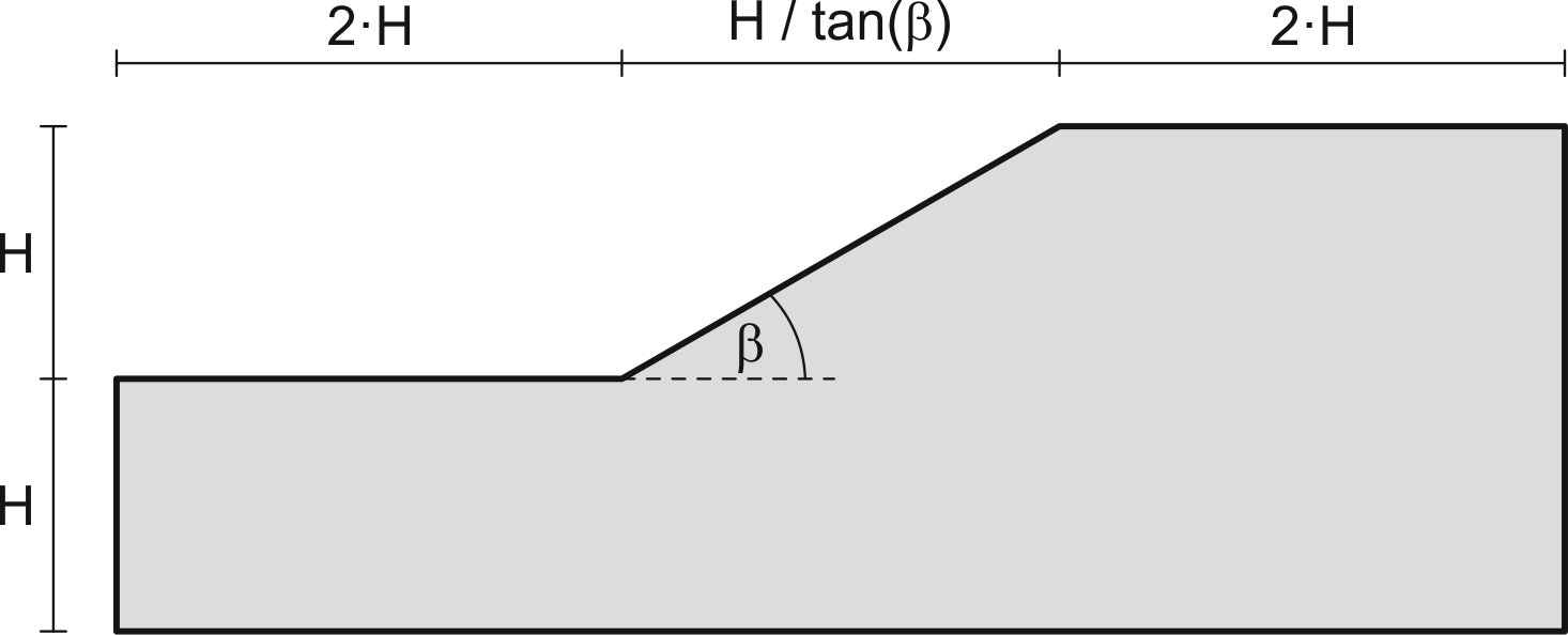
Figure 1. Geometry of the slope
The file containing the mesh (Slope-30-mesh.inp) is discussed first and then the step file (Slope-30.inp) is addressed.
Mesh
For the soil, two-dimensional u-solid finite elements are utilised to discretise the displacement u of the solid phase. The mesh is composed of 8-noded rectangle elements (termed u8-solid) with quadratic interpolation order.
.
.
*Element, Type = U8-solid
.
.
In the mesh file, node sets (NSet) and element sets (ElSet) have been defined to address groups of nodes and elements to be used in the step files (e.g. for the definition of boundary conditions). The following node sets have been defined in the mesh file and used in the step files: left, bottom, right, all. Only one element set has been defined: all.
Properties, Initial conditions and step definitions
The step file (Slope-30.inp) first includes the mesh file by defining:
*Include = Slope-30-mesh
As the slope is composed of a single homogeneous material, the solid section only covers one area and material:
*Solid Section, Elset = all, Material = MC
Materials
The material behavior of the soil is described by the Mohr-Coulomb model with material parameters selected as unit weight \(\gamma = 20\,\mathrm{kN/m}^3\), Young's modulus \(E = 30\,\mathrm{MPa}\), Poisson's ratio \(\nu = 0.2\), cohesion \(c=6\,\mathrm{kPa}\), friction angle \(\varphi=30^\circ\) and dilation angle \(\psi = 30^\circ\), where \(\varphi\) and \(\psi\) need to be inserted in radians. A transition lode angel of \(\theta_t = 29.5^\circ\) has been selected.
To consider that shear strength parameters of a specific material parameter set should be reduced in a strength reduction analysis, the keyword *Reducible Strength needs to be specified in the material definition.
*Material, name=MC, phases = 1

*Mechanical = MOHR-COULOMB
30000.0, 0.2, 6, 0.5236, 0.5236, 29.5

*Density
2.0

*Reducible Strength
Initial conditions
The initial conditions are defined in a way that the initial stress increases with increasing depth, approximating the stress state before the slope is created by excavation.
*Initial conditions, type = stress, Geostatic
all, 0, -400, 20, 0, 0.5, 0.5
Amplitudes
Amplitudes need to be defined to allow for changes of loads or boundary conditions during a step. For this example, only an unloading ramp is needed to incrementally decrease the reaction forces at the nodes in Step 2.
*Amplitude, name = UnloadingRamp, type = Ramp
0.0, 1.0, 1.0, 0.0
Steps
The first step is conducted in terms of a geostatic step. In this step, the initial stress distribution defined in the initial conditions is considered and deformations of all nodes are restricted in x- and y-direction, allowing for no deformations in the entire model. The reaction forces associated to the restricted degrees of freedom (DOF) at all nodes are saved. VTK output files are generated to allow for post-processing with Paraview. Note that the FoS should be selected as element output parameter for all steps of the simulation.
Step 1: Geostatic
*Step, name = step1, inc=1
*geostatic

*Body force, instant
all, grav, 10, 0, -1, 0

*Boundary
all, u1, 0.0d0
all, u2, 0.0d0

*Save reaction force
all, 2
*Save reaction force
all, 1

*Output, field, vtk, ascii
*Node output, nset = all
u
*Element output, elset = all
s, e, FOS

*End Step
Step 2: Excavation
The second step is performed as a static step. In this step, the reaction forces are gradually reduced to zero, allowing for the system to deform and find an equilibrium stress state by developing shear stresses. The boundary conditions are modified such that lateral deformations are restricted at the left and right boundaries and lateral and vertical deformations are restricted at the bottom boundary of the model.
*Step, name = step2, inc=200
*Static
0.05, 1., 0.005, 0.05

*Body force, instant
all, grav, 10.0, 0, -1, 0

*Boundary, op=new
left, u1, 0.
right, u1, 0.
bottom, u2, 0.
bottom, u1, 0.

*Reaction force, amplitude = UnLoadingRamp
all, 1
*Reaction force, amplitude = UnLoadingRamp
all, 2

*Output, field, vtk, ascii
*Node output, nset = all
u
*Element output, elset = all
s, e, FOS

*End Step
Step 3: Strength reduction
In the third step, a strength reduction analysis is conducted. Starting with an initial factor of safety of \(\text{FoS}_0 = 1.0\), the FoS is increased in each increment by \(\Delta\) \(\text{FoS}\). The maximum number of iterations is set to 16. SRM default convergence criteria are selected to 0.1, 0.1, 0.1, 1e-6, 1e-6, 1.0. To allow for the inspection of incremental displacements during post-processing (e.g. with Paraview), the *Reset option can used.
*Step, name = step3, inc=1000, maxiter=16
*Reduction
1.0, 0.05, 0.05, 1e-4

*Body force, instant
all, grav, 10.0, 0, -1, 0

*Boundary
left, u1, 0.
right, u1, 0.
bottom, u2, 0.
bottom, u1, 0.

*Reset
Displacement, Strain

*Controls, u, modify
0.01, 0.01, 0.01, 1e-6, 1e-6, 1.0

*Output, field, vtk, ascii
*Node output, nset = all
u
*Element output, elset = all
s, e, FOS

*End Step
Lastly, the step file is closed by the *End input statement.
*End input
Results
After the simulation is finished, the Slope-30.pvd file can be opened in Paraview to start the post-processing. The critical slip surface, as shown in Figure 2, is obtained by plotting the displacement magnitude at the last increment of the simulation.
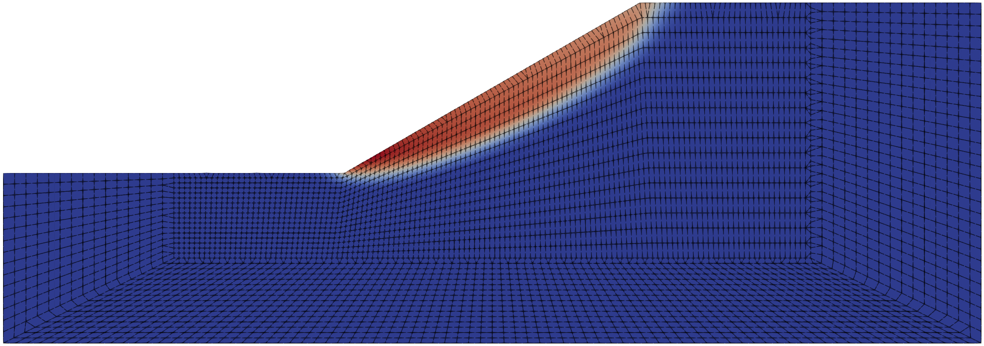
Figure 2. Critical slip surface (displacement magnitude) after safety analysis
The solution progress as well as the final FoS are saved in the *.sta file. In this example, the stability of the homogeneous slope is determined as FoS = 1.50.
Note that the estimation of the slope stability based on non-convergence might yield slight overestimation of the FoS. For this reason, it is emphasized to also inspcet the max. displacements vs. FoS plot. In this plot (Fig. 3), the critical FoS inidicating the level of safety of the slope under investigation can be identified by a sharp kink in the FoS vs. max. displacements plot for displacements plotted in logarithmic scale.
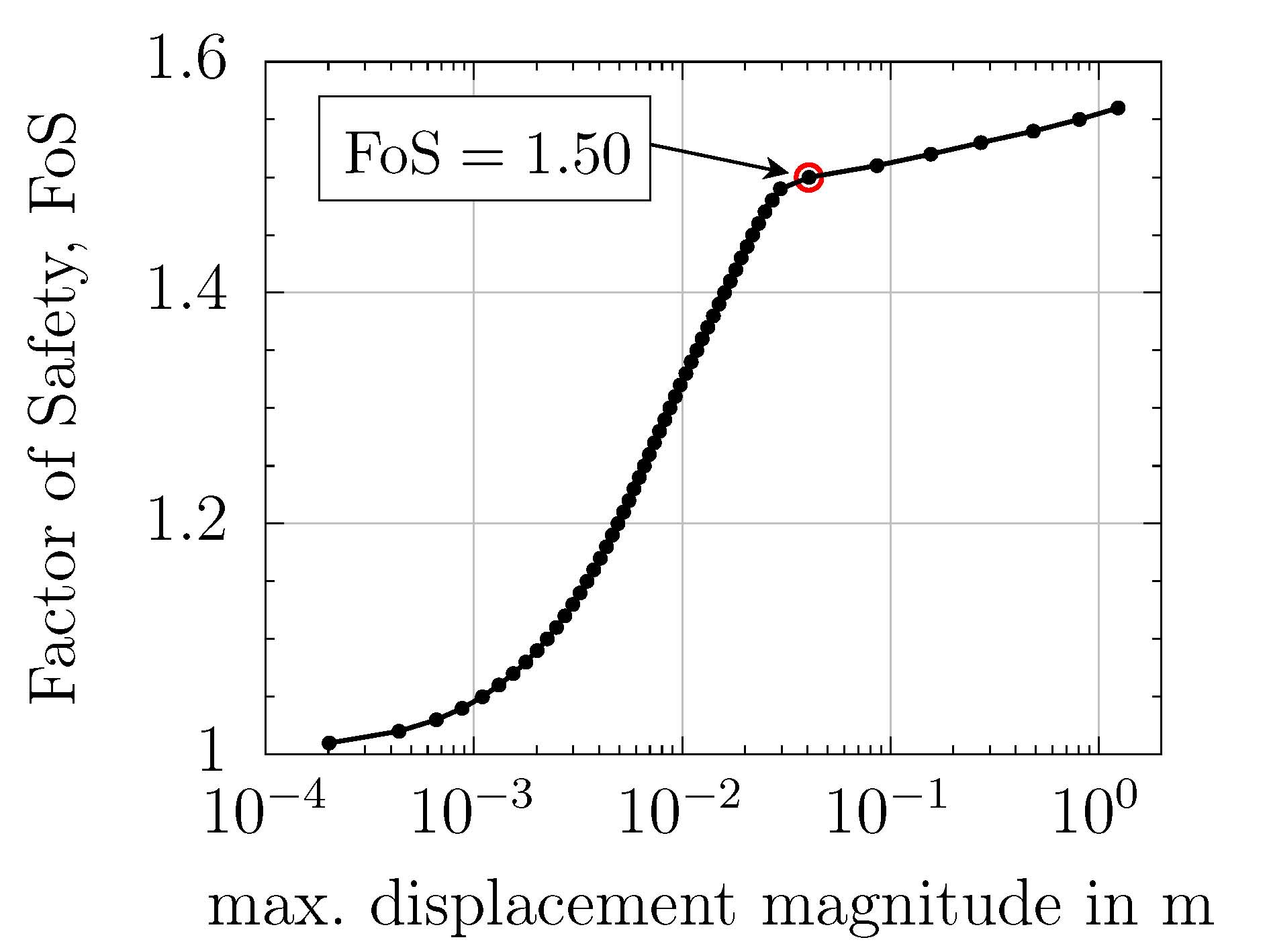
Figure 3. Max. displacement magnitude versus Factor of Safety (FoS)