1D site response: linear elastic (implicit and explicit time integration)
An incomplete input file that can be used as a starting point for this tutorial in combination with the finite element mesh can be downloaded here.
This first section of the 1D site response tutorial introduces some important features such as compliant base boundary conditions and multi-point constraints and their importance in 1D site response simulations. For this purpose we consider the soil column to consist of one homogeneous soil (the material of layer1, layer2, layer3 and layer4 are the same) and assuming linear elastic material behaviour.
In order to assess the accuracy of the implemented methods in numgeo, we first apply a single sinusoidal velocity signal at the base of the model. The target signal is displayed in Figure 1 and can be downloaded here

Figure 1. Sinusoidal target signal applied at the base of the model
The signal will propagate from the bottom of the model to the top surface. There it will be reflected and travels back in the direction of the bottom boundary. In order to avoid artificial reflections, a compliant base boundary condition is used to impose the signal. Contrary to the use of Dirichlet boundary conditions (i.e. prescribing the velocities at the nodes directly) an equivalent shear force will be applied to the bottom boundary. This boundary condition is designed such that a target signal can be enforced and at the same time reflections are prevented.
Surface definition
The compliant base boundary condition will be applied as a distributed surface load DSload. DSloads are applied to surfaces. To create a surface from a node set, we use the *Surface keyword in numgeo:
*Surface, name=bottom, type=node
soil.bottom
Material
As already stated in the introduction, the material is considered to be linear elastic. We assume a Young's modulus of \(E=10\) MPa and a Poisson's ratio of \(\nu = 0.25\), resulting in a shear modulus of \(4\) MPa. We use these - admittedly very low - values to allow the shaft to be properly tracked, even with the rather small model dimensions. As the focus here is on the general procedure and the introduction of individual functions, this is considered acceptable. The density of the solid grains and pore water are \(\rho^s=2.2\) t/m³ and \(\rho^w=1.0\), respectively.
*Material, Name = elastic, phases = 2

*Mechanical = Linear_Elasticity
1d4, 0.25

*Density
2.2, 1.0
The bulk modulus of pore water is assumed to be \(K^w=1.1\cdot 10^6\) kPa, which accounts for minor air inclusions in the ground water. The hydraulic conductivity is \(10^{-3}\) m/s and the dynamic viscosity is \(\mu^w=10^{-6}\)kPa\(\cdot\)s, resulting in a permeability of \(10^{-10}\) m².
*Bulk modulus
1.1d6

*Permeability = isotropic
1d-10

*dynamic viscosity
1d-6
Due to the single point integration of the element, zero energy modes (hourglass modes) can develop in the simulation and lead to spurious deformations rendering the simulation results useless. To counteract these spurious deformations, a stabilising hourglass stiffness is added:
*Hourglass, stiffness = 100
Amplitudes
The target signal is displayed in Figure 1. Such a signal could be realized using an in-build amplitude definition of numgeo (type = rising_sine). However, most earthquake signals are provided as tabular data. numgeo offers the possibility to read in such data as an amplitude using the type = tabular option of the amplitude keyword *Amplitude. In order not to include potential long lists of data in the main input file, we store the signal data in a separate file and load this file using the include statement:
*Amplitude, name = rising, type = tabular
*Include, input=signal-sinus
Note that the file with the signal has to be of type .inp and the file ending (inp) is omitted from the command statement as shown above. Subsequent to the excitation, we want to include a phase in the simulation where no further excitation is applied to the model, but the wave propagation is still followed. For this we define a second amplitude of zero magnitude over a long time period (10 seconds in the present case).
*Amplitude, name = zero, type = ramp
0.0, 0.0, 10.0, 0.0
Initial conditions
The initial void ratio is assumed to be \(e_0=1.0\) in the entire model. The initial effective stress follows a linear distribution with \(\sigma_v^\prime=0\) kPa at the top of the column and \(\sigma_v^\prime=-1600\) kPa at the bottom of the column (depth = 100 m). \(K_0=1.0\) is assumed. Similarly the initial pore water pressure at the top of the column (where the ground water level is located) is \(p^w = 0\) kPa and at the bottom of the column \(p^w=1000\) kPa. The corresponding input file command are given below.
*Initial conditions, type = void ratio, default
soil.all, 1.0

*Initial conditions, type = stress, geostatic
soil.all,  100., 0., 0., -600., 1., 1.

*Initial conditions, type = pore water pressure, default
soil.all, 0.0d0, 1000.0d0, 100.0d0, 0.0d0
Step 1: Geostatic
During the first step equilibrium between the stress from the self weight of the soil and the pore water and the initial conditions is established using a Geostatic step.
*Step, name=Geostatic, inc = 1
*Geostatic
The gravitation grav is assumed to be \(g=10\) m/s²:
*Body Force, instant
soil.all, grav, 10.d0, 0, -1, 0
The displacements nodes of the left and the right vertical boundary are constrained in horizontal direction, whereas the displacements of the nodes of the bottom boundary are constrained in vertical direction. The pore water pressure is prescribed at all nodes.
*Boundary
soil.bottom, u2, 0.0d0
soil.left, u1, 0.0d0
soil.right, u1, 0.0d0

*Boundary, hydrostatic
soil.all, pw, 10, 100
In the subsequent step we want to replace the horizontal boundary conditions to allow for the definition of multi-point constraints enforcing the desired 1D conditions. For this we store the reaction forces calculated at the horizontal boundary conditions:
*Save Reaction force
soil.all, 1
Finally we request to save selected simulation results such that we can visualize them later in Paraview and close the step using the *End Step keyword.
*Output, field, vtk, ASCII
*node output, nset = soil.all
U, V, A, pw
*element output, elset = soil.all
S, E

*End Step
Step 2: Multi-point constraints
The purpose of the second step is to replace the horizontal static (Dirichlet) boundary conditions by equivalent static forces. This can be done by applying the reaction forces stored in the previous step (*Reaction force, instant). No change in load is considered.
*Step, name=ReplaceBC, inc = 1
*Static
1., 1., 1., 1.

*Body Force, instant
soil.all, GRAV, 10.d0, 0, -1, 0

*Boundary
soil.bottom, u1, 0.0d0
soil.bottom, u2, 0.0d0

*Boundary, hydrostatic
soil.all, pw, 10, 100

*Reaction force, instant
soil.all, 1
Next the multi-point constraints (MPC) are set in place:
*Equation, EqualDOF
*penalty=1e8
soil.left, soil.right,u1
*Equation, EqualDOF
*penalty=1e8
soil.left, soil.right,u2
The *Equation, EqualDOF command is designed such that if more then one node is present in the assigned node sets, the displacements of the nodes with the shortest euclidean distance are coupled. This feature makes the application of MPC in site response analyses very convenient.
Finally we specify the output for this step and close the step
*Output, field, vtk, ASCII
*node output, nset = soil.all
U, V, A, pw
*element output, elset = soil.all
S, E

*End Step
Step 3: Excitation
In the third step we apply the excitation at the base of the model. This is done performing a Dynamic simulation, taking into account the effects of inertia:
*Step, name=Input, inc=10000
*Dynamic
0.001, 1, 0.001, 0.001
*Hilber-Hughes-Taylor = -0.05
The Hilber-Hughes-Taylor integration scheme is used to advance the solution in time. The numerical damping parameter \(\alpha\) controling the damping of high-frequency noise is set to -0.05, which corresponds to the recommended minimum value. The total step time is 1 second and time increments of \(\Delta t = 0.001\) s are used.
The body forces, static equivalent forces and MPCs are kept the same as in the previous steps. The displacements are only constrained in vertical direction at the bottom of the model. The pore water pressure is prescribed at the top of the model.
*Step, name=Input, inc=10000
*Dynamic
0.001, 1, 0.001, 0.001
*Hilber-Hughes-Taylor = -0.05

*Body Force, instant
soil.all, GRAV, 10.d0, 0, -1, 0

*Boundary
soil.bottom, u2, 0.
soil.top, pw, 0.0d0

*Reaction force, instant
soil.all, 1

*Equation, EqualDOF
*penalty=1e8
soil.left, soil.right,u1
*Equation, EqualDOF
*penalty=1e8
soil.left, soil.right,u2
The signal is applied using the previously introduced compliant base boundary condition with the amplitude signal read in as tabular data. The load is applied at the bottom surface in \(x\) (1) direction. The compliant base BC requires information about the impedance (\(\rho c_s\)) of the underlying material. In the present case, the shear wave velocity can be calculated as \(c_s = \sqrt{G/\rho}\). With \(G=4\) MPa and \(\rho=(1-n)\cdot 2.2 + n\cdot1 = 1.6\) t/m² it follows that \(c_s=50\) m/s and \(\rho c_s = 80\) t/(ms).
*Dsload, amplitude=rising
bottom, compliant, 1, 80
For the wave propagation we want to control the solution for each field (displacement and pore water pressure) separately. We therefore deactivate the global controls and activate the dof-based controls u and pw.
*Controls, global, deactivate
*Controls, u, activate
*Controls, pw, activate
Since the dynamic analysis consists of many small increments, we reduce the frequency with which the results are stored *Frequency = 10. In addition we define a print output to store more detailed output information for selected nodes (only the nodes of node set soil.left) at each increment.
*output, field, vtk, ASCII
*Frequency=10
*node output, nset = soil.all
U, V, A, pw
*element output, elset = soil.all
S, E

*output,print
*node output, nset=soil.left
U, V, A

*End Step
Step 4: Resting step
During the last step no further excitation is applied to the base of the model. We are only interested in the propagation of the waves already existing. For this, the only boundary condition that is changed is the compliant base boundary condition, where the amplitude is changed to the amplitude with zero magnitude: *Dsload, amplitude=zero. The complete definition of the step is given below.
*Step, name=Resting, inc=10000
*Dynamic
0.005, 10., 0.005, 0.005
*Hilber-Hughes-Taylor = -0.05

*Body Force, instant
soil.all, GRAV, 10.d0, 0, -1, 0

*Reaction force, instant
soil.all, 1

*Dsload, amplitude=zero
bottom, compliant, 1, 80

*Boundary
soil.bottom, u2, 0.0d0
soil.top, pw, 0.0d0

*Equation, EqualDOF
*penalty=1e8
soil.left, soil.right,u1
*Equation, EqualDOF
*penalty=1e8
soil.left, soil.right,u2

*Controls, global, deactivate
*Controls, u, activate
*Controls, pw, activate

*output, field, vtk, ASCII
*node output, nset = soil.all
U, V, A, pw
*element output, elset = soil.all
S, E

*output,print
*node output, nset=soil.left
U, V, A

*End Step
Results
There are many different quantities that can be evaluated from the simulation results. The one that we are focusing on in this example is the velocity \(v_x\) recorded at the bottom and the top of the model. Since the material model is linear elastic and no additional damping was defined, the amplitude of the velocity signal recorded at the top of the column is expected to be exactly twice the velocity recorded at the base of the model. The velocity at the base of the model should be exactly the target signal. Checking these requirements give information about the accuracy of the implementation. The results are given in Figure 2.
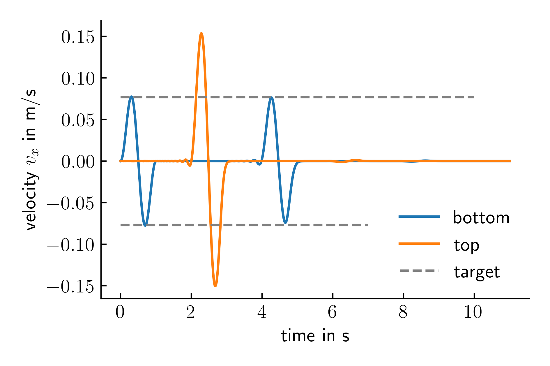
Figure 2. Recorded velocity at the bottom and the top of the model.
Python Skript for plotting the results
The python script used to generate Figure 2 is given below:
import numpy as np
import matplotlib.pyplot as plt

plt.rcParams['xtick.direction'] = 'in'
plt.rcParams['ytick.direction'] = 'in'
plt.rcParams['text.usetex'] = True
plt.rcParams['font.size'] = 12
plt.rcParams['axes.spines.right'] = False
plt.rcParams['axes.spines.top'] = False

def cm2inch(*tupl):
    inch = 2.54
    if isinstance(tupl[0], tuple):
        return tuple(i/inch for i in tupl[0])
    else:
        return tuple(i/inch for i in tupl)

directory = 'simulation-lin-print-out'

#
# Displacement top + bottom
#

plt.figure(figsize=cm2inch(12,8))

data = np.genfromtxt(directory+'/SOIL.LEFT_node_4.dat', skip_header=1)
plt.plot(data[:,0]-2., data[:,4], label='bottom')

data = np.genfromtxt(directory+'/SOIL.LEFT_node_10.dat', skip_header=1)
plt.plot(data[:,0]-2., data[:,4], label='top')

plt.hlines(0.077, 0, 10, ls='--', color='grey', label='target')
plt.hlines(-0.077, 0, 7, ls='--', color='grey')

plt.xlabel('time in s')
plt.ylabel('velocity $v_x$ in m/s')
plt.legend(loc='lower right', frameon=False)
plt.tight_layout()

plt.savefig('./time_velocity_bottom_top.pdf', dpi=400)
plt.savefig('./time_velocity_bottom_top.png', dpi=400)
Comparison with explicit time integration
For a simulation with explicit time integration, the element type is changed to
u4u4-red.
Because of the two phases, two hourglass stiffnesses are required:
*Hourglass, stiffness = 100, 100
Boundary conditions and reaction forces have to be adjusted in step 1:
*Boundary
soil.all, w1, 0.0d0
soil.all, w2, 0.0d0

*Save Reaction force
soil.all, 1
*Save Reaction force
soil.all, w1
And in step 2:
*Boundary
soil.bottom, w2, 0.0d0
soil.bottom, w1, 0.0d0

*Reaction force, instant
soil.all, 1
*Reaction force, instant
soil.all, w1

*Equation, EqualDOF
*penalty=1e8
soil.left, soil.right,w1
*Equation, EqualDOF
*penalty=1e8
soil.left, soil.right,w2
*explicit Dynamic
1d-9, 5,3d-5,3d-5

*Equation, EqualDOF
*penalty=1e8
soil.left, soil.right,w1
*Equation, EqualDOF
*penalty=1e8
soil.left, soil.right,w2
The comparison with the implicit solution is given below:
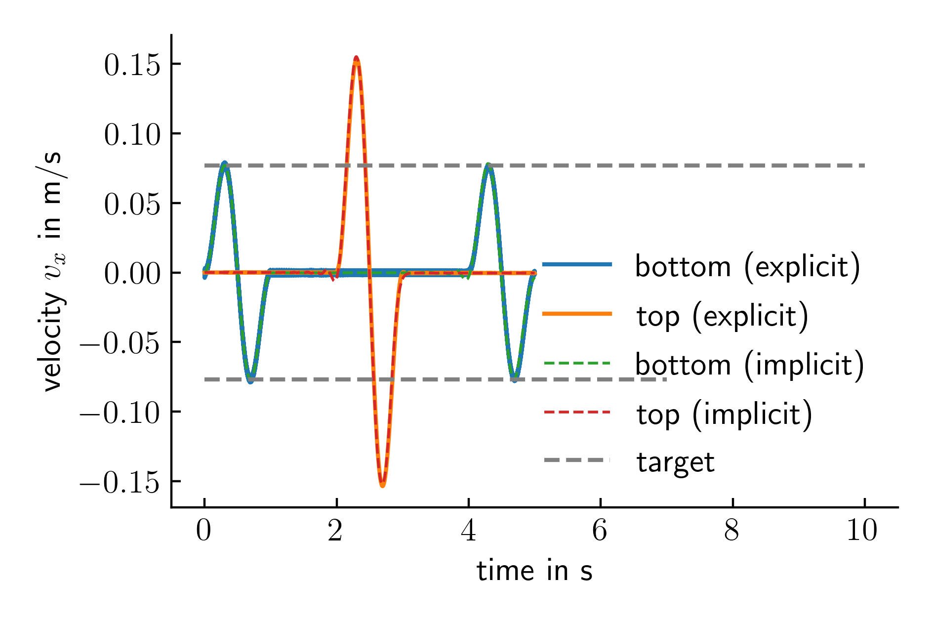
Figure 2. Recorded velocity at the bottom and the top of the model for explicit and implicit time integration.