Oedometric Compression Test

Development of geometry model and groups

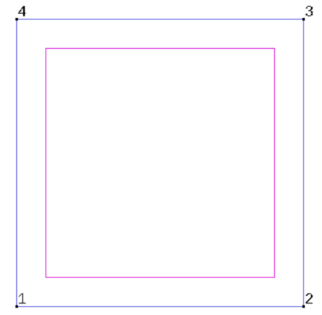
Creating a geometry is the first step to run a problem in numgeo with GiD. The shape can be made by using the straight line and entering exact coordinates into the command line.

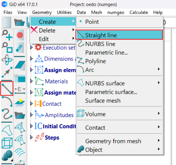
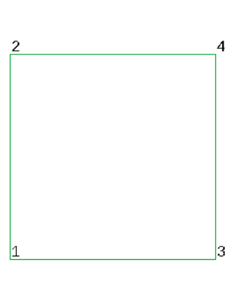
The following are the coordinates for the oedometric compression test.

0.0, 0.0
1.0, 0.0
1.0, 1.0
0.0, 1.0

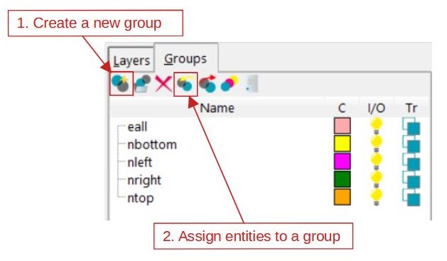
After entering all coordinates, the shape must be closed by clicking on the first point and joining it. Define the NURBS surface by selecting all lines and leave with ‘esc’.

Geometry oedometric test — Figure 2: Geometry of the model

Add all relevant groups by the tab on the right side. For the groups nleft, nright, ntop and nbottom select each nodes. For the group eall the complete surface needs to be elected.

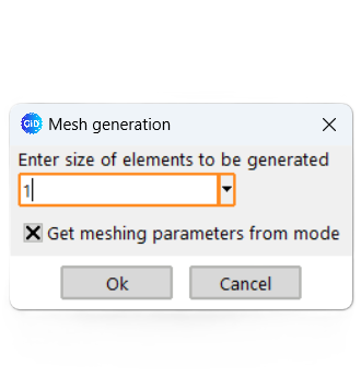
Creation of groups — Figure 3: Create groups of the model

Mesh generation

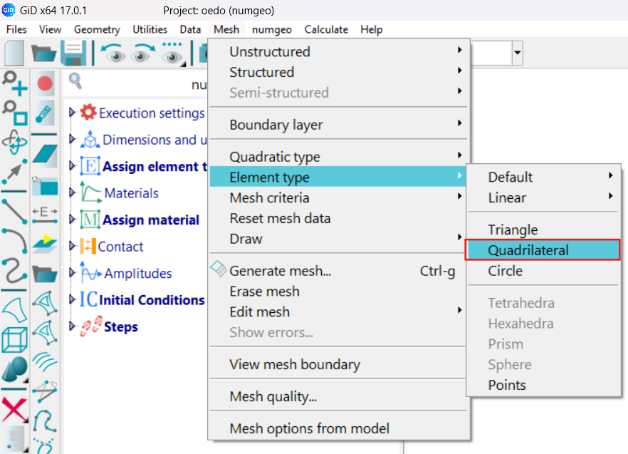
The element type for the mesh can be triangular, quadrilateral, or circular. A quadrilateral mesh element is defined in this test, since it is a quadratic geometry and only one mesh element is needed. Create the mesh by entering the element size of 1.0 m. For a better overview toggle the mesh-view using the button on the left bar.

Input definition

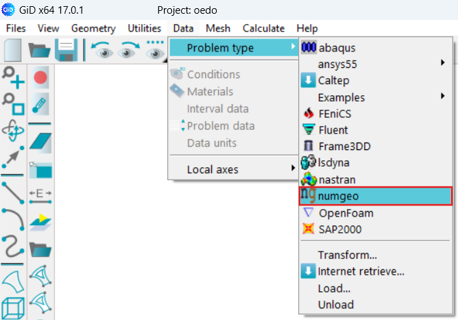
To add properties to the input file, the numgeo problem type must be loaded in GiD (Data -> Problem type -> numgeo). A list with all input elements will then be shown on the left side.

Choose problem type — Figure 5: Load numgeo problem type

Use the list in the left to navigate through the data tree and proceed in the order in which they are listed.

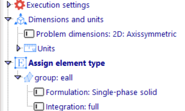
First, choose the right problem dimension (2D: Axisymmetric) and assign an element type (single-phase solid) for all elements.

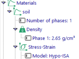
Figure 6: Dimension and element type of the model

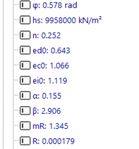
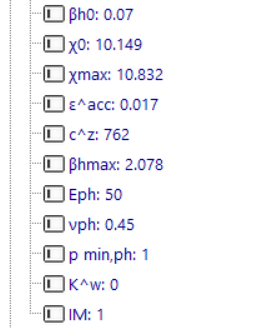
Define the material name 'soil', the number of phases and the density of the material. Next, choose the material model under Stress-Strain and define the listed material parameters. Then assign the material to all elements.

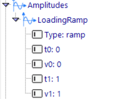
Firgure 7: Material model and properties

Next, we define the amplitude as a ramp and change the name to 'LoadingRamp'. The default values are correct for the oedometric compression test.

Define an amplitude — Firgure 8: Amplitude for an oedometric compression test

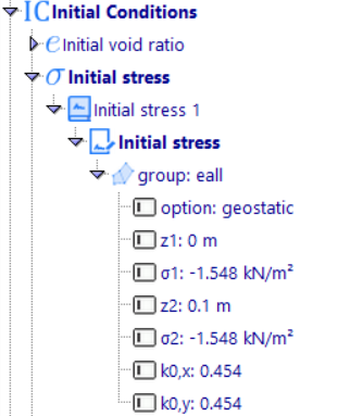
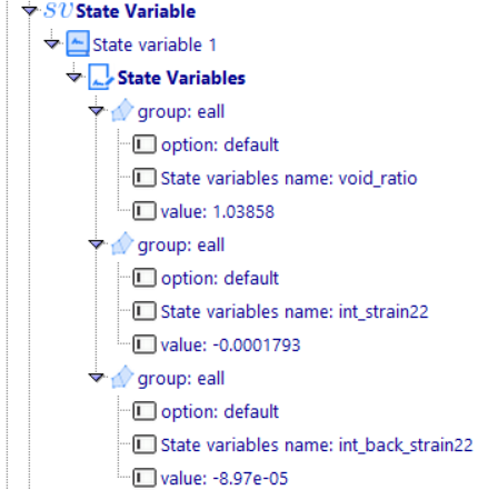
The initial stress and three state variables must be applied for this element test to all elements. For the state variables, the name of every variable must be typed in with the corresponding value.

initial conditions — Firgure 9: Initial conditions for an oedometric compression test

Step 1: Geostatic

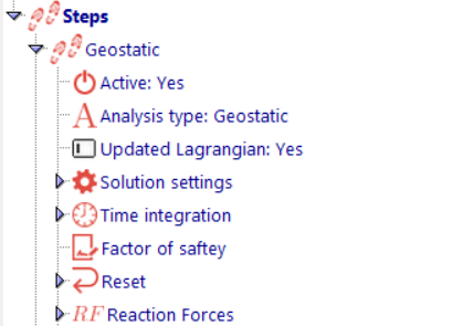
Finally, the steps can be defined. For the first step change the name of the step to 'Geostatic' and enter the number of increments. Since we only have one increment in this step, the default values for maximum and minimum iterations can be neglected.
Change the analysis type also to geostatic.

Firgure 10: Geostatic step for an oedometric compression test

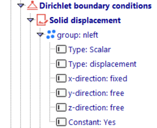
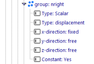
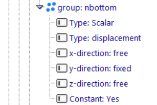
Below the tab ‘ Dirichlet boundary conditions’ the solid displacements in both directions can be defined. Therefore, fix the displacements in the x-direction of nleft and nright and in the y-direction for nbottom.

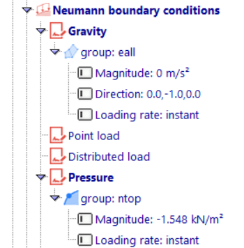
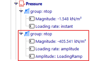
Firgure 11: Displacement boundaries for an oedometric compression test

Apply the gravity force to all elements. The default values are already given there. In addition to the gravity force, define a pressure of -1.548 kN/m² on the top with an instant loading rate.

Firgure 12: Initial loads for an oedometric compression test

Since this is a basic simulation, only print output for all elements is requested for stress, strain, and void ratio.

Step 2: Loading

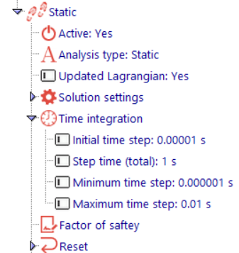
For the second step, copy the first step (with assigned groups) and change the name to ‘Loading’. Also change the number of increments and the analysis type. Now the input of time integration is unlocked.

Static step — Firgure 13: Loading step for an oedometric compression test

The boundary conditions do not change in the loading step.
In addition to the initial loads, a pressure of -405.541 kN/m² on the top with a loading rate of the previously defined amplitude needs to be applied.

Pressure for static step — Firgure 14: Secondary loads for an oedometric compression test

The output requirements also remain the same as in the geostatic step.

Results and visualization

Save the file in a folder, where the problem should run and start the calculation process (numgeo -> Generate numgeo files). numgeo will automatically create two input files and start calculating. Once the calculation process is finished, the results can be plotted using python for example.

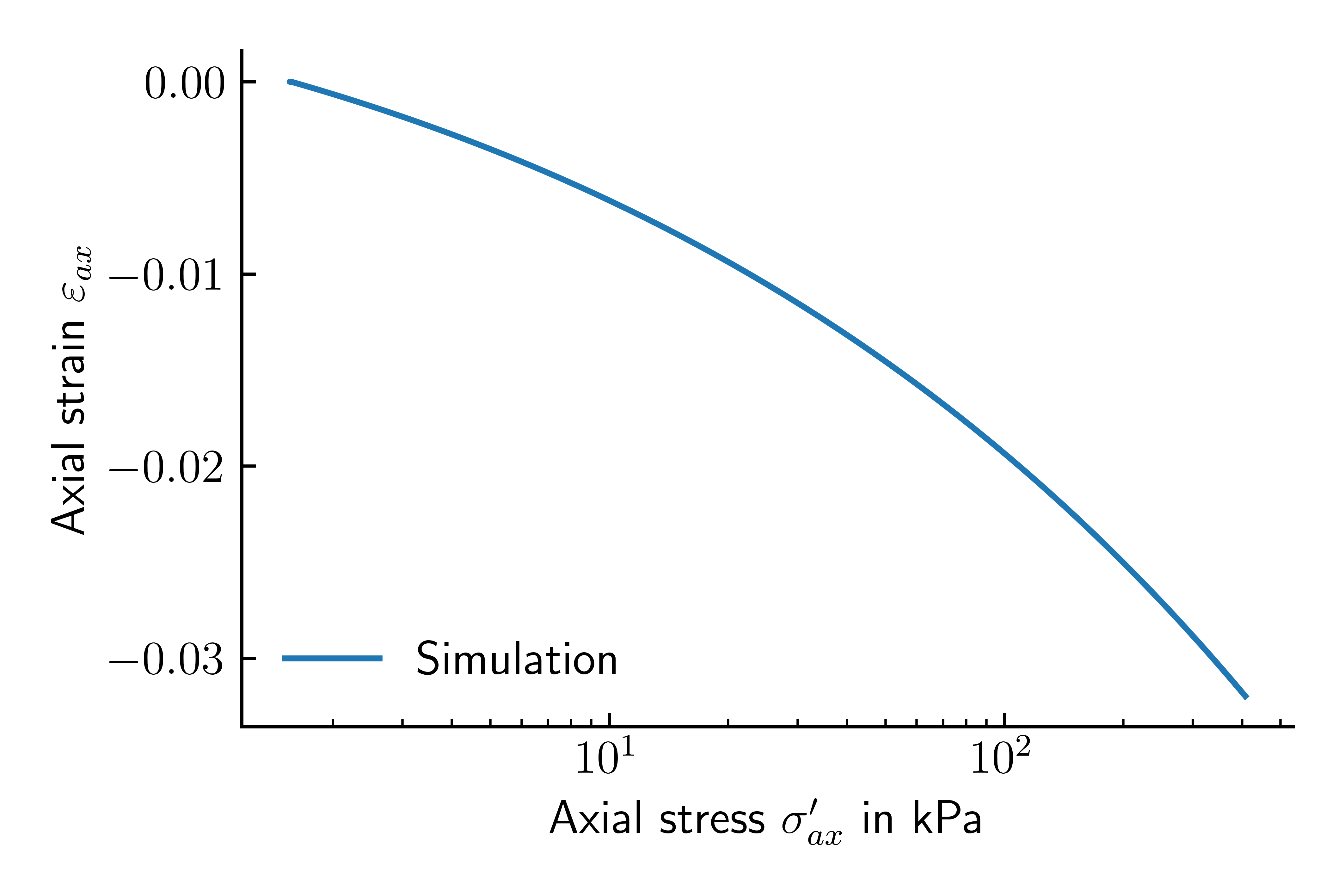
The following Python script was used to plot the data shown in figure 15.

import numpy as np
import matplotlib.pyplot as plt

plt.rcParams['xtick.direction'] = 'in'
plt.rcParams['ytick.direction'] = 'in'
plt.rcParams['text.usetex'] = True
plt.rcParams['font.size'] = 12
plt.rcParams['axes.spines.right'] = False
plt.rcParams['axes.spines.top'] = False

def cm2inch(*tupl):
    inch = 2.54
    if isinstance(tupl[0], tuple):
        return tuple(i/inch for i in tupl[0])
    else:
        return tuple(i/inch for i in tupl)

sim = np.genfromtxt('./oedo-print-out/EALL_element_1.dat', skip_header=1)

plt.figure(figsize=cm2inch(12,8))
plt.semilogx(-sim[:,2], sim[:,8], label='Simulation')
plt.xlabel('Axial stress $\sigma_{ax}^\prime$ in kPa')
plt.ylabel('Axial strain $\\varepsilon_{ax}$')
plt.legend(loc='lower left', frameon=False)
plt.tight_layout()

plt.savefig("stress-strain",dpi = 900)

Result of the simulation — Firgure 15: Result of the oedometric compression test

For more information please refer to the corresponding numgeo tutorial for the Oedometric Compression Test.