Undrained cyclic triaxial test
Development of geometry model
The first step in configuring a problem in numgeo with GiD involves creating the geometry of the model. For this, use the straight line ![]() or enter exact coordinates into the command line.
The following coordinates are used for the undrained cyclic triaxial test, as we only consider one simple element in this tutorial.
or enter exact coordinates into the command line.
The following coordinates are used for the undrained cyclic triaxial test, as we only consider one simple element in this tutorial.
0.0, 0.0
1.0, 0.0
1.0, 1.0
0.0, 1.0
The relevant groups must be added before creating the mesh. The groups will be shown on the tab on the right side. For the groups nleft, nright, ntop and nbottom select each nodes. For the group eall the complete surface needs to be elected.
Mesh generation
In this test, a quadrilateral mesh element is chosen because the geometry is quadratic, requiring only one mesh element. Create the mesh by entering the element size of 1.0 m. For a better overview toggle the mesh-view using the button ![]() on the left bar. Speed up the mesh creation using 'CTRL+G'.
on the left bar. Speed up the mesh creation using 'CTRL+G'.
Input definition
To add properties to the input file, the numgeo problem type ![]() must be loaded in GiD (Data -> Problem type -> numgeo). A data tree will then be shown on the left side. Now, use the data tree in the left to navigate through the settings and proceed in the order in which they are listed.
must be loaded in GiD (Data -> Problem type -> numgeo). A data tree will then be shown on the left side. Now, use the data tree in the left to navigate through the settings and proceed in the order in which they are listed.
- First, choose the right problem dimension
 (2D: Axisymmetric) and assign an element type
  (single-phase solid) for all elements.
 - Define the material name 'soil', the number of phases and the density of the material. Next, choose the material model under Stress-Strain
 and define the listed material parameters. Then assign the material
  to all elements.
For the undrained cyclic triaxial test the material parameters of Hypoplasticity + Intergranular Strain Anisotropy are defined as follows:
| parameters | value | parameters | value | |
|---|---|---|---|---|
| \( φ \) | 0.578 rad | \( β_{h0} \) | 0.07 | |
| \( h_s \) | 9958000 kN/m² | \( χ^0 \) | 10.149 | |
| \( n \) | 0.252 | \( χ^{max} \) | 10.832 | |
| \( e_{d0} \) | 0.643 | \( ϵ^{acc} \) | 0.017 | |
| \( e_{c0} \) | 1.066 | \( c^{z} \) | 762.0 | |
| \( e_{i0} \) | 1.119 | \( β_{hmax} \) | 2.078 | |
| \( α \) | 0.155 | \( E_{ph} \) | 50.0 | |
| \( β \) | 2.906 | \( ν_{ph} \) | 0.450 | |
| \( m_R \) | 1.345 | \( p_{min,ph} \) | 1.0 | |
| \( R \) | 0.000179 | \( K^{ω} \) | 0.0 0.0 kN/m² |
- Next, we define the amplitude
 with the name 'loading-signal' of type lab-cyclic-stress-strain-control. You will find this type under type -> additional amplitudes -> lab cyclic loading. Add the values given below in the tab and apply it to all elements.
Amplitude 'loading-signal':
lab-cyclic-stress-strain-control
- stress component:
s11-s22- stress 1:
40- stress 2:
-40- rate:
-1e-5- N:
35
- The initial stress
 and some state variables
  must be applied for this element test to all elements. For the state variables, the name of every variable must be typed in with the corresponding value. The values for all initial conditions are given below:
Initial stress:
- option:
geostatic- \( z_1 \):
0.0- \( σ_1 \):
-99.3- \( z_2 \):
0.1- \( σ_2 \):
-99.3- \( k_{0,x} \):
1.0- \( k_{0,y} \):
1.0State variables:
- void_ratio:
0.716- int_strain11:
-0.0001035- int_strain22:
-0.0001035- int_strain33:
-0.0001035- int_back_strain11:
-5.18e-05- int_back_strain22:
-5.18e-05- int_back_strain33:
-5.18e-05
Step 1:  Loading
- The next step involves defining the simulation phase. Rename this step to 'Loading' and enter the number of increments of 10000000.
- Change the analysis type
 to static. Now the input of time integration
  is unlocked. The following values for time integration are used:
- Initial time step:
1 s- Time step (total):
10000000 s- Minimum time step:
0.01 s- Maximum time step:
1 s
- Below the tab '
 Dirichlet boundary conditions’ the solid displacements in both directions can be defined. Fix the displacements in the x-direction of nleft and in the y-direction for nbottom.
 - In addition, the linear increasing vertical displacement of the top nodes is prescribed to 1. Similiar to that, the linear increasing hotizontal displacement of the right nodes is prescribed to -0.5. Note: Select Loading-signal for the amplitude, as this is a non-constant displacement.
- Apply the gravity force to all elements. The default values are already given there. In addition to the gravity force, define a pressure of -99.3 kN/m² on the top and a pressure of -99.3 kN/m² on the right side, both with an instant loading rate.
- Since this is a basic simulation, only print output
 for all elements is requested for stress, strain, and void ratio with a frequency of 2.
Results and visualization
Save the file in a folder, where the problem should run and start the calculation process (numgeo -> Generate numgeo files). numgeo will automatically create two input files and start calculating. After completing the calculations, results can be visualized using tools like python for detailed analysis.
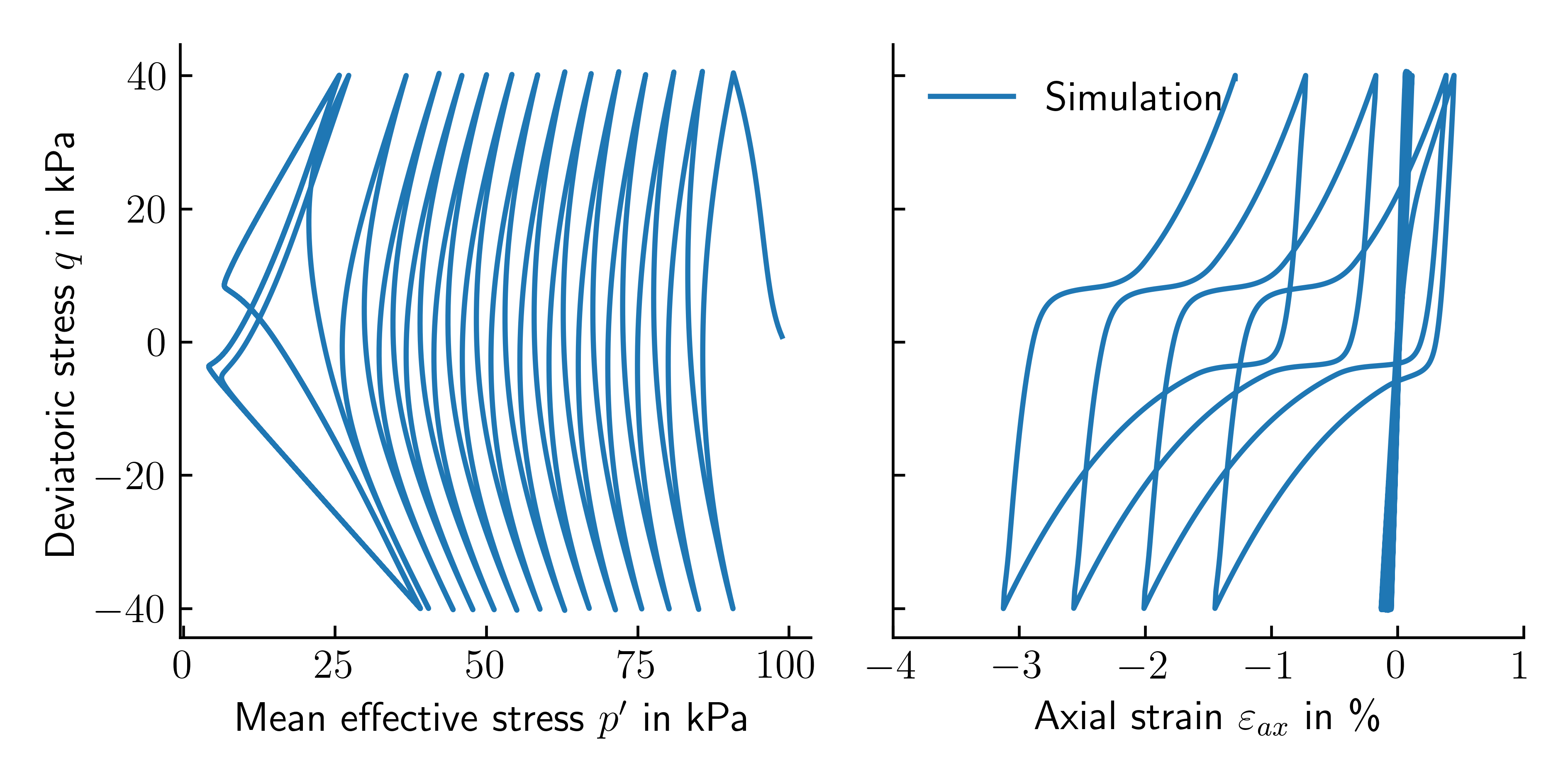
The following Python script was used to plot the data shown in figure 1.
import numpy as np
import matplotlib.pyplot as plt

plt.rcParams['xtick.direction'] = 'in'
plt.rcParams['ytick.direction'] = 'in'
plt.rcParams['text.usetex'] = True
plt.rcParams['font.size'] = 12
plt.rcParams['axes.spines.right'] = False
plt.rcParams['axes.spines.top'] = False

def cm2inch(*tupl):
    inch = 2.54
    if isinstance(tupl[0], tuple):
        return tuple(i/inch for i in tupl[0])
    else:
        return tuple(i/inch for i in tupl)

sim = np.genfromtxt('./undr-cyclic-print-out/EALL_element_1.dat', skip_header=1)


fig, (ax1,ax2) = plt.subplots(ncols=2, sharey=True, figsize=cm2inch(16,8))

ax1.plot(-(sim[:,1]+sim[:,2]+sim[:,3])/3.-sim[:,-1], -(sim[:,2]-sim[:,1]), label='Simulation')
ax1.set_ylabel('Deviatoric stress $q$ in kPa')
ax1.set_xlabel('Mean effective stress $p^\prime$ in kPa')

ax2.set_xlabel('Axial strain $\\varepsilon_{ax}$ in \%')
ax2.plot(-sim[:,8]*100, -(sim[:,2]-sim[:,1]), label='Simulation')
ax2.legend(loc='upper left', frameon=False)
plt.xlim(-4,1)

fig.tight_layout()

plt.savefig('./triaxCUcyc-exp-vs-sim1.png', dpi=600)
plt.show()
For more information please refer to the corresponding numgeo tutorial for the Undrained cyclic triaxial test.