Undrained cyclic triaxial test using HCA model

Development of geometry model

The first step in configuring a problem in numgeo with GiD involves creating the geometry of the model. For this, use the straight line or enter exact coordinates into the command line. The following coordinates are used for the undrained cyclic triaxial test with the HCA model, as we only consider one simple element in this tutorial.

0.0, 0.0
0.05, 0.0
0.05, 0.1
0.0, 0.1

After entering all coordinates, the shape must be closed by clicking on the first point and joining it. Define the NURBS surface by selecting all lines and leave with ‘esc’.

Mesh generation

In this test, a quadrilateral mesh element with quadratic nodes is chosen, as we require only one mesh element. For this, click on quadratic type -> quadratic to ensure a double amount of nodes. Then create the mesh by entering the element size of 0.1 m. For a better overview toggle the mesh-view using the button on the left bar. Speed up the mesh creation using 'CTRL+G'.

Input definition

To add properties to the input file, the numgeo problem type must be loaded in GiD (Data -> Problem type -> numgeo). A data tree will then be shown on the left side.

Groups can be assigned either before or during the navigation of the data tree. The groups will be shown on the tab on the right side. For the groups nleft, nright, ntop and nbottom select each line. For the group eall the complete surface needs to be elected.

Now, use the data tree in the left to navigate through the settings and proceed in the order in which they are listed.

Predefined strain ampiltude

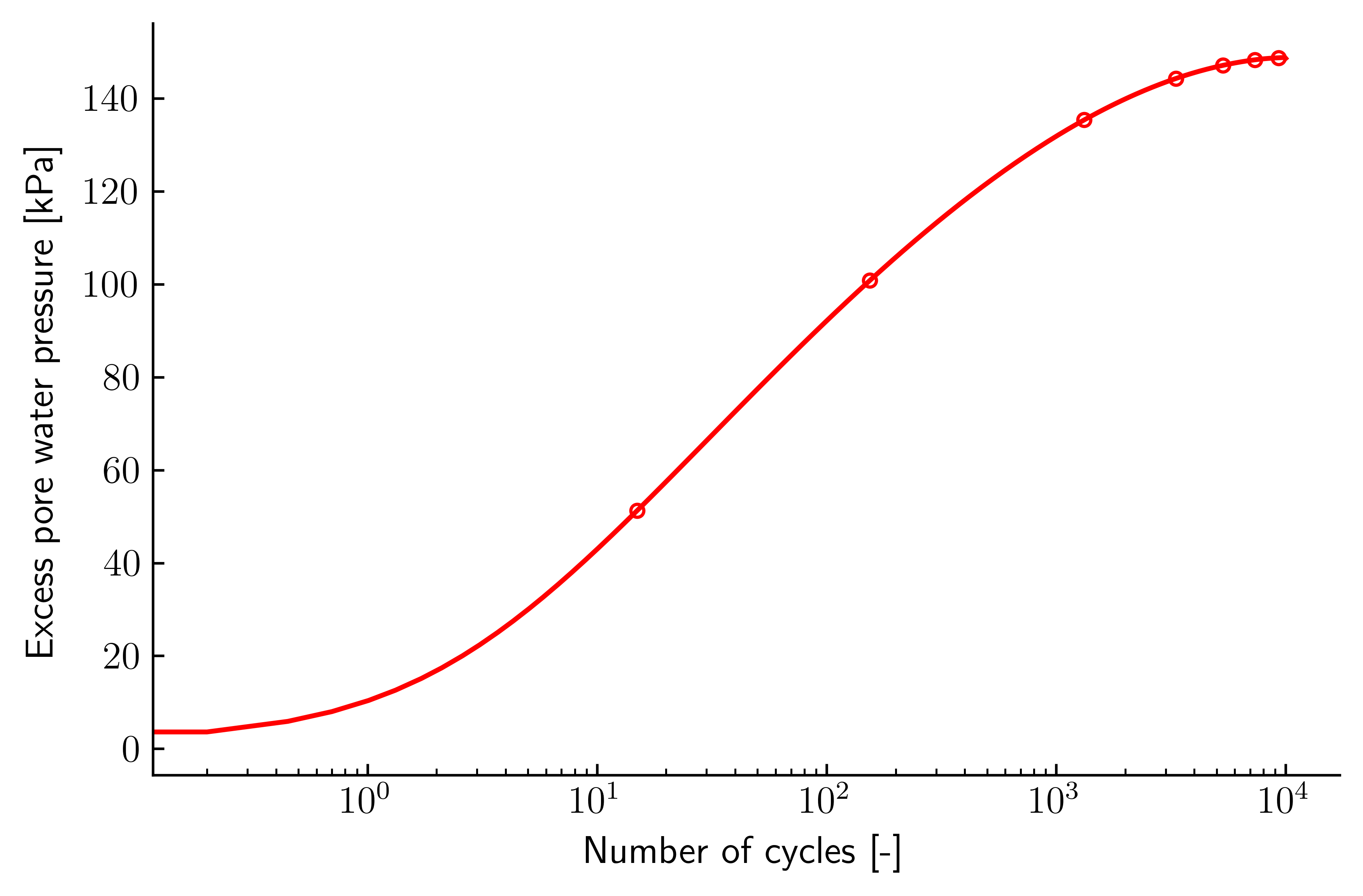
In the first example, the strain amplitude is not calculated by a conventional constitutive model, but a measured amplitude from an experiment is used. This is typically the case if the simulations are performed to calibrate or check the parameters of the HCA model.

First, choose the right problem dimension (2D: Axisymmetric) and assign an element type (two-phase-u-p) with full integration for all elements.
Define the material name 'soil', the number of phases of 2 and the density of both phases.

Density:

Phase 1: 2.65 g/cm³

Phase 2: 1 g/cm²

Next, choose the material model under Stress-Strain and define the listed material parameters.

For the undrained cyclic triaxial test with the HCA model the material parameters of linear elasticity are defined as follows:

parameters	value
\(E\)	5000 kN/m²
\( ν\)	0.32

Activate the HCA model under stress-strain (HCA) and define the material parameters for the High Cycle Accumulation (HCA) model. The period of the cycles is 1. The properties for the HCA model are as follows:

parameters	value	parameters	value
\( C_{N1} \)	0.000295	\( C_{Pi3} \)	0
\( C_{N2} \)	0.41	\( p_{atm} \)	100 kN/m²
\( C_{N3} \)	1.9e-05	\( e_{ref} \)	1.054
\( C_{ampl} \)	1.33	\( ϵ_{ref}^{ampl} \)	0.0001
\( C_e \)	0.6	\( A \)	1209
\( C_p \)	0.23	\( a \)	1.63
\( C_Y \)	1.68	\( n \)	0.5
\( C_{Pi1} \)	0	\( ν \)	0.32
\( C_{Pi2} \)	0	\( φ_c \)	0.578

In addition to the material parameters, the HCA model requires the declaration of the step types. The first step is a low-cycle ("implicit") step. The actual HCA phase is performed in step HCA.

Implicit HCA steps: Geostatic

Recording HCA steps: HCA

Explicit HCA steps: HCA

The bulk modulus of the pore water and the permeability have to be defined. In numgeo, the permeability equals the dynamic viscosity (set to \(10^{-6}\) kPa) multiplied with the hydraulic conductivity and divided by the unit weight of water (\(γ_{w}\) = 10 kN/m³).

Permeability (isotropic): \(1e^{-12}\)

Bulk modulus of fluid phases: 2.2 kN/m²

Dynamic viscosity: \(1e^{-6}\)

Now, assign the material to all elements.
The initial stress and some state variables must be applied for this element test to all elements. For the state variables, the name of every variable must be typed in with the corresponding value. The values for all initial conditions are given below:

Initial void ratio:

0.818

Initial stress:

option: geostatic

\( z_1 \): 0.0

\( σ_1 \): -150

\( z_2 \): 0.1

\( σ_2 \): -150

\( k_{0,x} \): 1.0

\( k_{0,y} \): 1.0

State variables:

void_ratio: 0.818

strain_ampl: 3e-04

Step 1: Geostatic

The next step involves defining the simulation phase. Rename this step to 'Geostatic' and enter the number of increments of 1.
Change the analysis type to geostatic.
Below the tab ' Dirichlet boundary conditions’ the solid displacements in both directions can be defined. Fix the displacements in the x-direction of nleft and in the y-direction for nbottom.
In addition, apply the boundary for pore water pressure for all nodes (nall):

Pore water pressure:

Type: Linear distribution

Type: Increment

Gradient: 0.1

Zero level: 0.0

Apply the gravity force to all elements with a magnitude of 10 m/s² and the given direction. In addition to the gravity force, define a pressure of -150 kN/m² on the top and a pressure of -150 kN/m² on the right side, both with an instant loading rate.
There is no output requested for this step.

Step 2: HCA

For the second step, copy the first step (with assigned groups) and change the name to ‘HCA’. Also change the number of increments to 10000000 and the analysis type to transient. Now the input of time integration is unlocked. The following values for time integration are used:

Initial time step: 0.2 s

Time step (total): 10000 s

Minimum time step: 0.0001 s

Maximum time step: 100 s

The existing input for solid displacement, gravity and pressure remain the same. The boundary condition for pore water pressure must be deleted to ensure an excess pore water pressure.
For the print element output stress, strain, void ratio and 'strain_ampl' is requested for all elements. We also need the print node output for the top nodes to plot the results afterwards.

Calculating strain amplitude

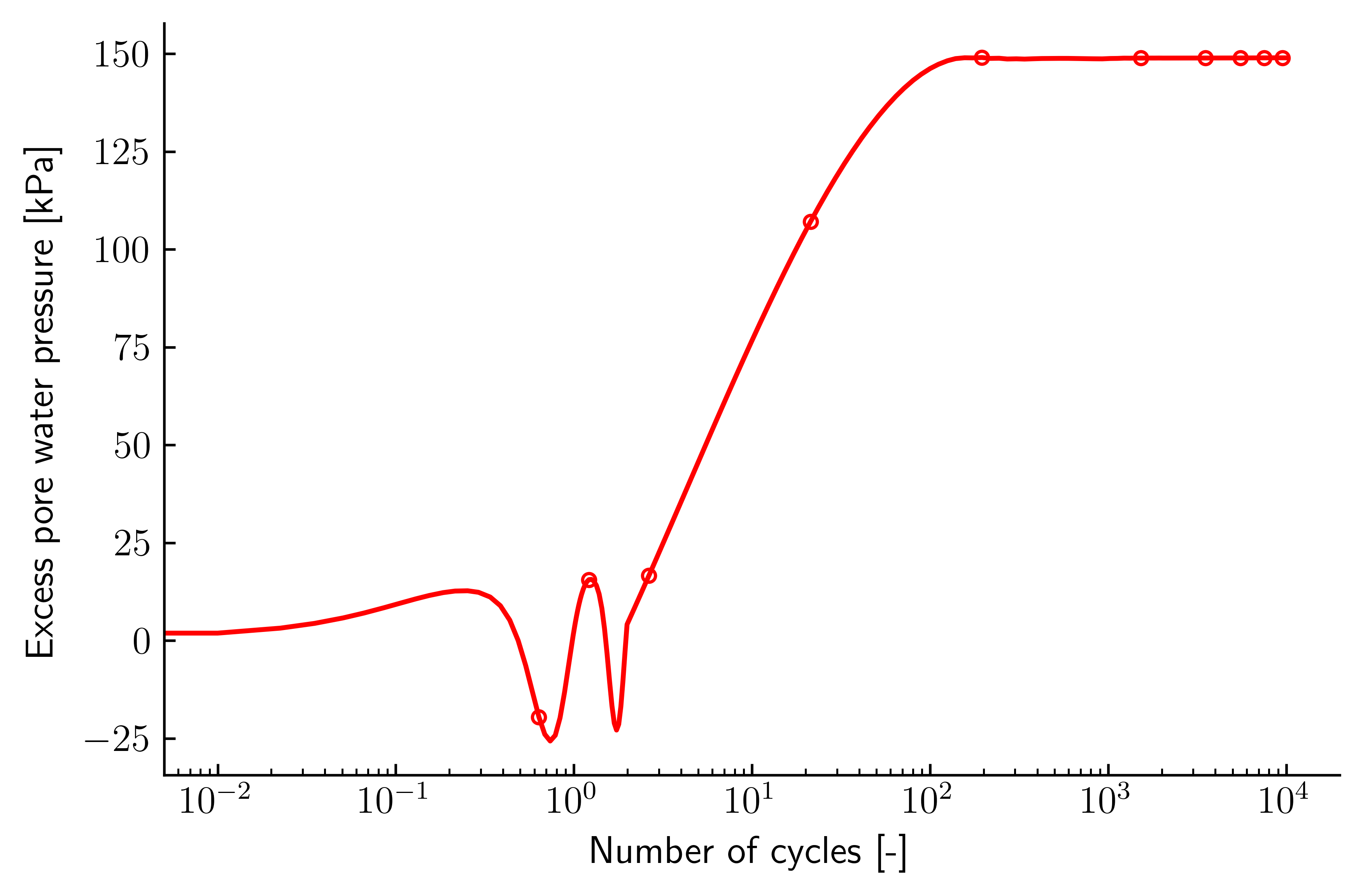
In the second example, the strain amplitude is calculated by a conventional constitutive model, the hypoplastic model with intergranular strain extension in the present case. Having to calculate the strain amplitude is the case for a typical boundary value problem.

To enter this second example in numgeo.gid, the first file is copied and the following changes are made:

Change the material model to 'Hypoplastic + IGS' and enter the following material parameters:

parameters	value	parameters	value
\( φ \)	0.577 rad	\( β \)	2.5
\( ν \)	0.0	\( m_T \)	1.2
\( h_s \)	4000000 kN/m²	\( m_R \)	2.4
\( n \)	0.27	\( R \)	0.0001
\( e_{d0} \)	0.677	\( β_{R} \)	0.1
\( e_{c0} \)	1.054	\( χ \)	6.0
\( f_{ei0} \)	1.15	\( K^{ω} \)	0.0 kN/m²
\( α \)	0.14

The first two steps are low-cycle ("implicit") steps. The sinusoidal load is applied in FirstCycle and in SecCycle, whereby the strain curve is recorded for the latter. The actual HCA phase is performed in the step named HCA.

Implicit HCA steps: Geostatic, FirstCycle

Recording HCA steps: SecCycle

Explicit HCA steps: HCA

Next, we define the amplitude with the name 'sine1Hz' of type periodic. Add the values given below in the tab and apply it to all elements.

Amplitude 'sine1Hz': periodic

\(N\): 1

\(A_0\): 0

\(t_0\): 0

\(ω\): 6.283

\(A_i, B_i\): 0, 1

The initial conditions will remain the same in this example.

Step 1: Geostatic

The geostatic step remains unchanged. The input is explained in the first example.

Step 2: FirstCycle

Copy the 'HCA'-step with assigned groups, rename this step to 'FirstCycle' and enter the number of increments of 10000000.
The following values for time integration are used:

Initial time step: 0.01 s

Time step (total): 1 s

Minimum time step: 0.0001 s

Maximum time step: 0.05 s

In addition to the previously defined pressures, apply a pressure of -60 kN/m² on the top with an amplitude loading rate. Choose sine1Hz for the amplitude.
For the print element output stress, strain, void ratio and 'strain_ampl' is requested for all elements.

Step 3: SecCycle

Copy the 'FirstCycle'-step and change the name of the third step to 'SecCycle'. All other input parameters remain the same as in 'FirstCycle'.

Step 4: HCA

The HCA step remains unchanged. The input is explained in the first example.

Results and visualization

Save both files in a folder, where the problem should run and start the calculation process (numgeo -> Generate numgeo files). numgeo will automatically create two input files for each problem and start calculating. After completing the calculations, results can be visualized using tools like python for detailed analysis.

The following python script was used to plot the data for both examples shown in figure 1 and 2.

import matplotlib
import matplotlib.pyplot as plt
import matplotlib.ticker as mtick
from pylab import genfromtxt
from matplotlib import rc
import os 
import numpy as np
dir_path = os.path.dirname(os.path.realpath(__file__))
plt.rcParams['backend'] = "pdf"
plt.rcParams['xtick.direction'] = 'in'
plt.rcParams['ytick.direction'] = 'in'
plt.rcParams['text.usetex'] = True
plt.rcParams['font.size'] = 12
plt.rcParams['axes.spines.right'] = False
plt.rcParams['axes.spines.top'] = False
plt.rcParams['axes.linewidth'] = 0.8 

#=============================================================================
# Read data
#%% =============================================================================

sim1 = genfromtxt('linear_elasticity.gid/linear_elasticity-print-out'+'/'+'NTOP_node_3.dat',skip_header=1)
sim2 = genfromtxt('hypo.gid/hypo-print-out'+'/'+'NTOP_node_3.dat',skip_header=1)

#=============================================================================
# Plot first data
#%% =============================================================================
plt.figure(1)
plt.subplot(111)

plt.semilogx(sim1[:,0]-sim1[0,0],sim1[:,1],'or-',\
         markersize=4,markerfacecolor='none',markevery=20,\
         label=r'Simulation',clip_on=True)

ax = plt.gca()
ax.set_xlabel(r'Number of  cycles [-]')
ax.set_ylabel(r'Excess pore water pressure [kPa]',labelpad=7)

plt.tight_layout() 
fig = plt.gcf()  
fig.savefig('excess_pore_water_pressure_input_epsampl_linear_elasticity.png', dpi=600 , bbox_inches='tight')

#=============================================================================
# Plot second data
#%% =============================================================================
plt.figure(2)
plt.subplot(111)

plt.semilogx(sim2[:,0]-sim2[0,0],sim2[:,1],'or-',\
         markersize=4,markerfacecolor='none',markevery=20,\
         label=r'Simulation',clip_on=True)

ax = plt.gca()
ax.set_xlabel(r'Number of  cycles [-]')
ax.set_ylabel(r'Excess pore water pressure [kPa]',labelpad=7)

plt.tight_layout() 
fig = plt.gcf()  
fig.savefig('excess_pore_water_pressure_input_epsampl_hypo.png', dpi=600 , bbox_inches='tight')

Result of the simulation — Firgure 1: Excess pore water pressure versus number of load cycles for calculating the strain amplitude

For more information please refer to the corresponding numgeo tutorial for the Undrained cyclic triaxial test using HCA model.