Seepage of water through dam

Development of the numerical model

The first step is to create the geometry. This is done using the Straight-Line tool , where the model boundaries can be drawn by entering the exact coordinates in the command line. Accurate geometry is essential, as closed lines later form surfaces that represent the domain to be meshed and analyzed using the finite element method.

The coordinates for the numerical model are as follows:

Subsoil:

0,0 
80,0
80,2
0,2

Core:

32,2
48,2
44,13
36,13

Left core body:

8.5,2
36,13
32,2

Right core body:

71.5,2
44,13
48,2

After entering all the given coordinates for the subsoil, core, left core body, and right core body, each shape must be closed by connecting the last point back to the first point. Once the model is created, the lines should be intersected. This can be done by clicking Geometry → Edit → Intersection → Lines and then selecting the entire model. This step ensures that all regions share common nodes, which is essential for correct mesh generation.

Figure 1: Intersection tool in GiD

Next, create NURBS surfaces by selecting the boundary lines of each region and pressing Esc. Repeat this process for all parts of the dam (subsoil, core, left core body, and right core body), ensuring that each section is represented as an individual surface.

Figure 2: Creating a NURBS surface in GiD

Figure 3: Geometry of the dam model after defining surfaces

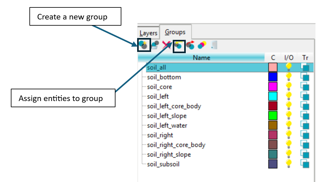
Next, groups are created by assigning either nodes, lines or surfaces to them. For the groups soil_bottom, soil_left, soil_left_slope, soil_right_slope, soil_left_water, and soil_right, the corresponding lines must be selected and for the groups soil_all, soil_core, soil_left_core_body, soil_right_core_body, and soil_subsoil, the complete surfaces should be selected. This is done by creating a new group and then assigning the appropriate nodes, lines, or surfaces as required.

Figure 4: Groups defined in the model

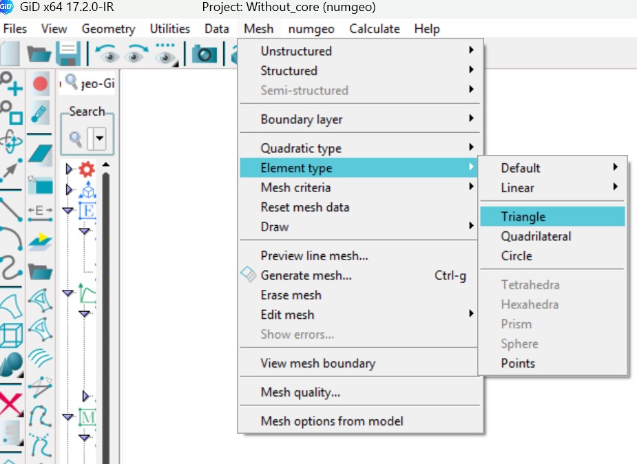
Then, 2-Dimensional finite element mesh was generated in numgeo-GiD. A triangular mesh with 6-noded elements (u6p3) was chosen. Create the mesh by setting the element size to 1.0 m. For a clearer view of the generated mesh, toggle the mesh display using the mesh-view icon on the left toolbar.

Figure 5: Generating triangular mesh

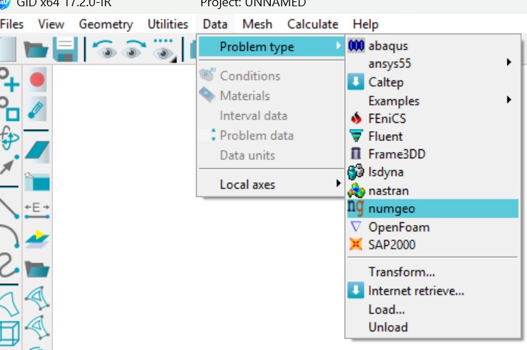
To define the model properties, first load the numgeo problem type in GiD by navigating to Data → Problem type → numgeo.

Figure 6: Loading numgeo problemtype

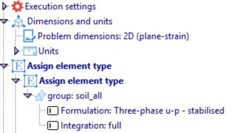
Set the problem dimension to 2D (Plane strain), and assign element 3-phase u-p stabilized formulation with full integration to soil_all, which enables the simultaneous consideration of soil, water, and air phases.

Figure 7: Assigning dimension and element type

Materials properties

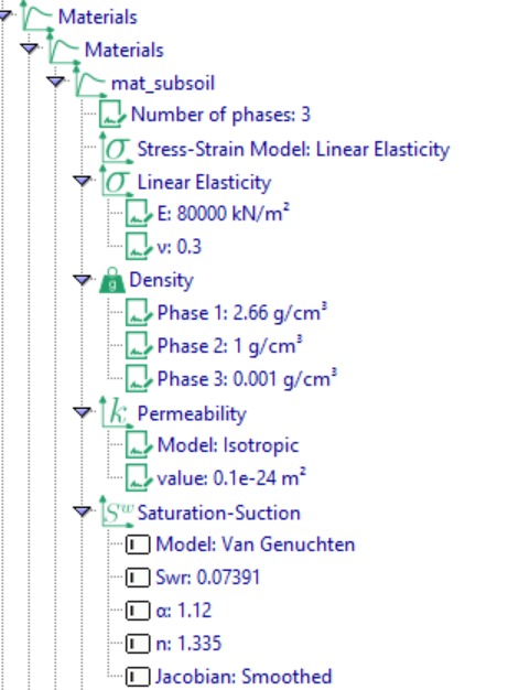
Next, we define the material properties. Under Material Definition, create a material named “mat_subsoil” and specify its parameters, including the number of phases, stress–strain model, density, permeability, saturation–suction relationship, permeability–saturation relationship, Bishop’s effective stress, bulk modulus, and dynamic viscosity, as shown in Figure 9.

Figure 9: Material parameters of subsoil

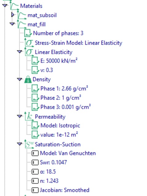
Next, we define material properties to fill, as shown in Figure 10.

Figure 10: Material parameters of fill

Assign materials

Next, we assign the materials. This step involves specifying the defined material properties to the corresponding sections that form the dam embankment.

Figure 11: Assign material

Initial conditions

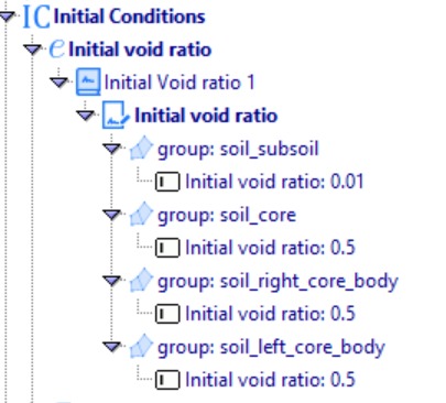
The next step is to define the initial conditions for the dam model. The initial void ratio values are set as follows: soil_subsoil = 0.01, soil_core = 0.5, soil_right_core_body = 0.5, and soil_left_core_body = 0.5. The very low value of 0.01 for the subsoil indicates a nearly impervious material, whereas the core and surrounding fill are assigned a higher void ratio of 0.5, reflecting their more permeable nature in the absence of a central core.

Figure 12: Initial void ratio

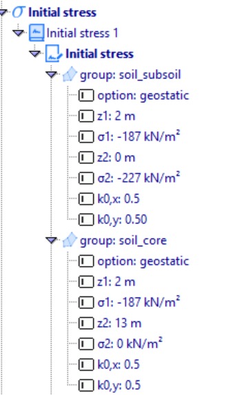
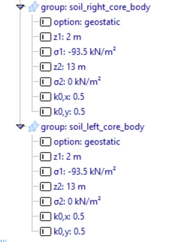
Next, the initial stress is assigned at the integration points of each element set. Geostatic stresses are introduced to simulate the soil’s self-weight.

Figure 13: Initial stress

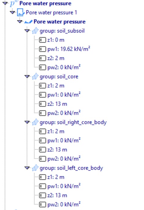
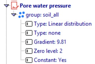
Finally, the initial pore water pressure is defined.

Figure 14: Initial pore water pressure

Simulation steps

Step 1

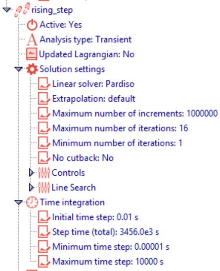
The next step is to define the geostatic step for the dam model. This step applies gravity loading to account for the self-weight of the dam materials, ensuring a realistic initial stress state before applying transient reservoir loads. Set the analysis type to Geostatic and specify the increment as 1.

Figure 15: Geostatic step

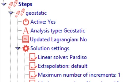
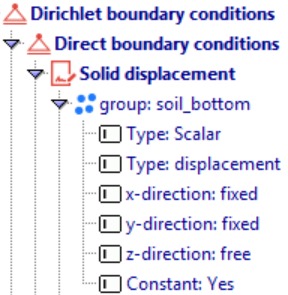
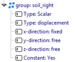
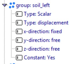
Under the Dirichlet boundary conditions tab , fix the soil_bottom in both the horizontal and vertical directions, while the sides (soil_left and soil_right) are fixed only in the horizontal direction.

Figure 16: Displacement boundary conditions

Next we define pore water pressure.

Figure 17: Pore water boundary conditions

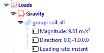
Apply a gravity load of 9.81 m/s² in the downward direction (0.0, -1.0, 0.0) to the soil group “soil_all”, using an instant loading rate for the geostatic procedure.

Figure 17: Pore water boundary conditions

Next, we assign the output. The model output is specified in VTK ASCII format with a frequency of 1. For the group Soil_all, the node results include displacements (u) and pore water pressure (pw), while the element results include stresses (S) and strains (E).

Step 2

In this stage, the loading step simulates the rising water level in the reservoir using a transient analysis. The step is defined as transient with a large number of increments (1,000,000) to accurately capture the gradual increase in water level over time. The displacement boundary conditions remain the same as those specified in the geostatic step.

Figure 18: Rising water

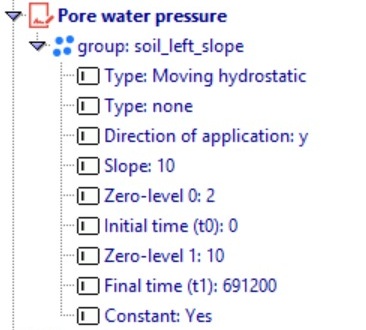
Next, we define the rising water. The upstream water supply is simulated by applying pore water pressure (pw) at the nodes in soil_left_water and soil_left_slope. The water level rises gradually over the first 8 days and then remains constant at 8 m. The boundary conditions are defined using a moving hydrostatic type in the slope direction, with both the zero-level and final-time pressures specified. This setup ensures that the soil is subjected to the correct hydraulic load from the upstream water body, reflecting realistic seepage conditions.

Figure 19: Moving hydrostatic for rising water level

For this loading step, the output is defined in VTK ASCII format with a frequency of 20. For the nodes in soil_all, the recorded results include displacement (u) and pore water pressure (pw). For the elements in soil_all, the results include stresses (S), strains (E), effective saturation (sat_eff), Darcy velocities (darcy_w1, darcy_w2), and saturation (sat).

After all steps have been defined, save the model to ensure that the current configuration is stored. Numgeo input files can then be generated by going to the Numgeo section and selecting Generate Files. Once the files are created, go to the Calculate section and click Calculate to run the numerical analysis. After the calculation is complete, the results can be visualized in ParaView for post-processing and interpretation.

Figure 20: Generating numgeo files

Results

Case I: Dam without core

After conducting the simulation, the position of the phreatic surface was recorded over time. The phreatic surface is defined as the region where the degree of saturation equals one. The contours corresponding to zero pore water pressure and full saturation illustrate the variation of pore water pressure with time. The results clearly indicate that water seeps into the embankment.

Figure 21: Pore water pressure and saturation at different simulation times.

Case II: Dam with core

An additional core material (mat_core) was introduced to simulate an impermeable barrier within the dam. The inclusion of this core significantly modifies the seepage behavior, reducing pore water pressures in the downstream region and effectively controlling the position of the phreatic line. Comparing this configuration with Case 1 (the dam without a core) highlights the critical role of the core in minimizing seepage through the embankment.

Figure 22: Core material properties and material assignment.

Figure 23: Pore water pressure and saturation at different simulation times.