Features of constitutive models for soils

Developing constitutive models for soils is challenging. The stress-strain behaviour of soils is in general highly non-linear, inelastic and depends on a series of state variables such as the current stress state, the density or the loading history, amongst many other. An (incomplete) overview of important aspects of constitutive models for soils is given in Figure 1. The most important ones will be discussed in the subsequent sections.

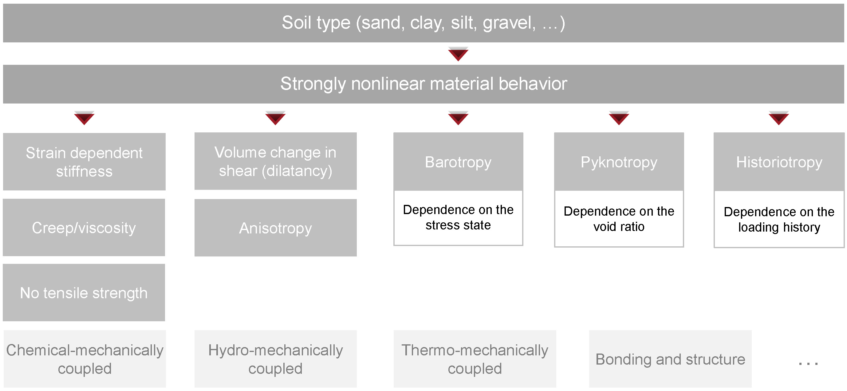Figure 1. Overview of important features of constitutive models for geotechnical engineering

For the sake of simplicity the important features are discussed in one-dimensional representations of the stress-strain relationships

Effective stress

Most constitutive models for soils are formulated in terms of effective stress which controls the mechanical behaviour of soils. An exception to this is the simulation of ideally undrained states with simple constitutive models. Here, a simulation with total stresses can be performed - the exact conditions required for this and the implications of these simulations are discussed in the Lecture Numerical Simulations in Geotechnical Engineering.

Irreversibility and loading history

One important soil property is the irreversibility of deformation. In other words, the soil skeleton does not return to its original shape after a load reversal. The only exceptions are extremely small deformations (e.g. as discussed in Basics of Soil Dynamics). In contrast to the fully reversible behaviour depicted in Figure 2a, which shows a clear relationship between stress and strain, irreversible behaviour requires the stiffness to be different during loading and unloading (Figure 2b). An important consequence of irreversibility is the absence of a clear relationship between stress and strain. An example of this is the results of an oedometric compression test with loading and unloading (see Figure 2c), where for a given axial strain there are two possible axial stresses and vice versa.

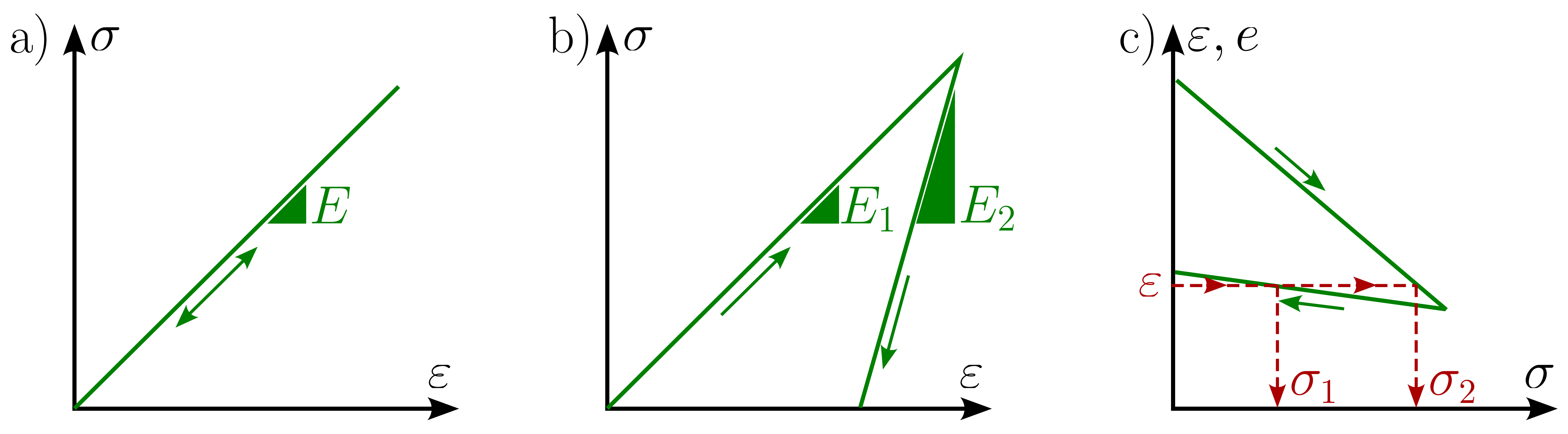Figure 2. a) reversible stress-strain relation, b) irreversible stress-strain relation, c) typical results from an oedometric compression test with loading and unloading.

for the case of reversible stress-strain relations depicted in Figure 2.a) the constitutive model calculating stress \(\sigma\) from strain \(\varepsilon\) can be formulated as follows:

\[ \sigma = E \varepsilon \]

where the constant \(E\) is the proportionality factor between stress and a parameter of the constitutive model.

Since changes in load direction can occur at any time, constitutive models for soils must be formulated as incremental stress-strain relationships:

\[ \Delta \sigma = E \Delta \varepsilon \]

where \(\Delta \sigma\) and \(\Delta \varepsilon\) are the stress and strain increments, respectively. More common is the formulation of the constitutive models in rate form:

\[ \dot{\sigma} = E\dot{\varepsilon} ~~~ \text{where}~~~ \dot{\sigma} = \dfrac{\partial \sigma}{\partial t} \approx \dfrac{\Delta \sigma}{\Delta t} ~~~ \text{and}~~~ \dot{\varepsilon} = \dfrac{\partial \varepsilon}{\partial t} \approx \dfrac{\Delta \varepsilon}{\Delta t} \]

Obviously, the stiffness \(E\) is not a constant anymore since it depends on the loading direction (see Figure 2b). This condition can be introduced in the constitutive model as follows:

\[ \dot{\sigma} = \begin{cases} E_1 \dot{\varepsilon} & ~~\text{if}~~ \dot{\varepsilon} > 0 \\ E_2 \dot{\varepsilon} & ~~\text{else} \end{cases} \]

Avoiding switching between loading and unloading

Above equation requires switching (if ... else ...) between loading and unloading. From an implementation point of view this requires the detection of load reversal - which in some cases might lead to numerical instabilities. From a mathematical point of view, switching between equations is not directly a problem, but it is rather inelegant. A more elegant formulation of the above equation is²

\[ \dot{\sigma} = \dfrac{E_1 + E_2}{2} \dot{\varepsilon} + \dfrac{E_1 - E_2}{2} |\dot{\varepsilon}| = E_{I} \dot{\varepsilon} + E_{II} |\dot{\varepsilon}| \]

therein, \(|\dot{\varepsilon}|\) is the absolute value of the strain rate. For \(\dot{\varepsilon} > 0\) and \(\dot{\varepsilon} = |\dot{\varepsilon}|\) above equation results in:

\[ \dfrac{E_1}{2} \dot{\varepsilon} + \dfrac{E_2}{2} \dot{\varepsilon} + \dfrac{E_1}{2} \dot{\varepsilon} - \dfrac{E_2}{2} \dot{\varepsilon} = E_1 \dot{\varepsilon} \]

while for unloading \(\dot{\varepsilon} < 0\) and \(\dot{\varepsilon} = -|\dot{\varepsilon}|\)

\[ - \dfrac{E_1}{2} |\dot{\varepsilon}| - \dfrac{E_2}{2} |\dot{\varepsilon}| + \dfrac{E_1}{2} |\dot{\varepsilon}| - \dfrac{E_2}{2} |\dot{\varepsilon}| = - E_2 |\dot{\varepsilon}| = E_2 \dot{\varepsilon} \]

is obtained. This approach is fundamental for the hypoplastic constitutive models. In elasto-plastic constitutive models, the reversible part of the deformation is usually considered elastic.

Nonlinearity

Another key feature of (most) constitutive models for soils is the non-linear relation between stress and strain. In other words, the incremental stiffness

\[ E = \dfrac{\dot{\sigma}}{\dot{\varepsilon}} \]

changes during the loading or unloading process. The reason for this is the influence of the current soil state on the stiffness. As the state of the soil changes in the course of loading or unloading, its stiffness also changes. The non-linearity of stiffness can be observed for example from the results of an oedometric compression test as shown in the animated Figure 3.

Figure 3. oedometric compression test on sand with loading and unloading.

The current state of a soil can be described by various variables. The state variables that should be taken into account by a "good" constitutive model for soils are the stress \(\sigma\) and the void ratio \(e\) (as a measure of relative density density):

\[ \dot{\sigma} = E(\sigma,e)\dot{\varepsilon} \]

For cohesive soils, the over-consolidation ratio OCR is sometimes used instead of the void ratio. A very simple example of a constitutive model that takes into account the influence of the effective stress \(\sigma\) and the void ratio \(e\) on the stiffness reads

\[ \dot{\sigma} = E_{ref} f_p f_e \dot{\varepsilon} ~~~\text{with:} ~~~ f_p = \left( \dfrac{\sigma}{\sigma_{ref}} \right)^{n_\sigma} ~~~ \text{and} ~~~ f_e = \dfrac{1+e}{e} \]

Above equation has three parameters: the reference stiffness \(E_{ref}\) evaluated at a given reference pressure \(\sigma_{ref}\) and the exponent \(n_\sigma\) controlling the increase of stiffness with increasing effective stress. The stress \(\sigma\) and the void ratio \(e\) are state variables in above equation and will evolve during loading and unloading.

Stress dependence

The influence of stress state on soil stiffness can be roughly divided into two parts: (1) the influence of mean effective stress \(p^\prime\) and (2) the influence of stress ratio \(\eta=q/p\). Details on the meaning and calculation of the invariants \(p\) and \(q\) are given in Section Invariants

The effect of mean effective stress is also known as Barotropy. As the mean effective stress increases, the stiffness of the soil also increases. We have already seen this for the results of oedometric compression tests in Figure 3, where the non-linear strain versus stress curve is a consequence mainly of the increase in stress. Similar observations can be made evaluating the results of drained monotonic triaxial tests in terms of the Stiffness \(E_{50}\). \(E_{50}\) is defined as the secant stiffness evaluated at 50% of the maximum deviatoric stress \(q_{50} = q_{max}/2\):

\[ E_{50} = \dfrac{q_{50}}{\varepsilon_{1,50}} \]

where \(\varepsilon_{1,50}\) is the axial strain corresponding to \(q_{50}\). Evaluating \(E_{50}\) on results from a series of drained monotonic triaxial tests with different initial mean effective stresses \(p_0^\prime\) clearly show the effect of barotropy as illustrated in Figure 4.

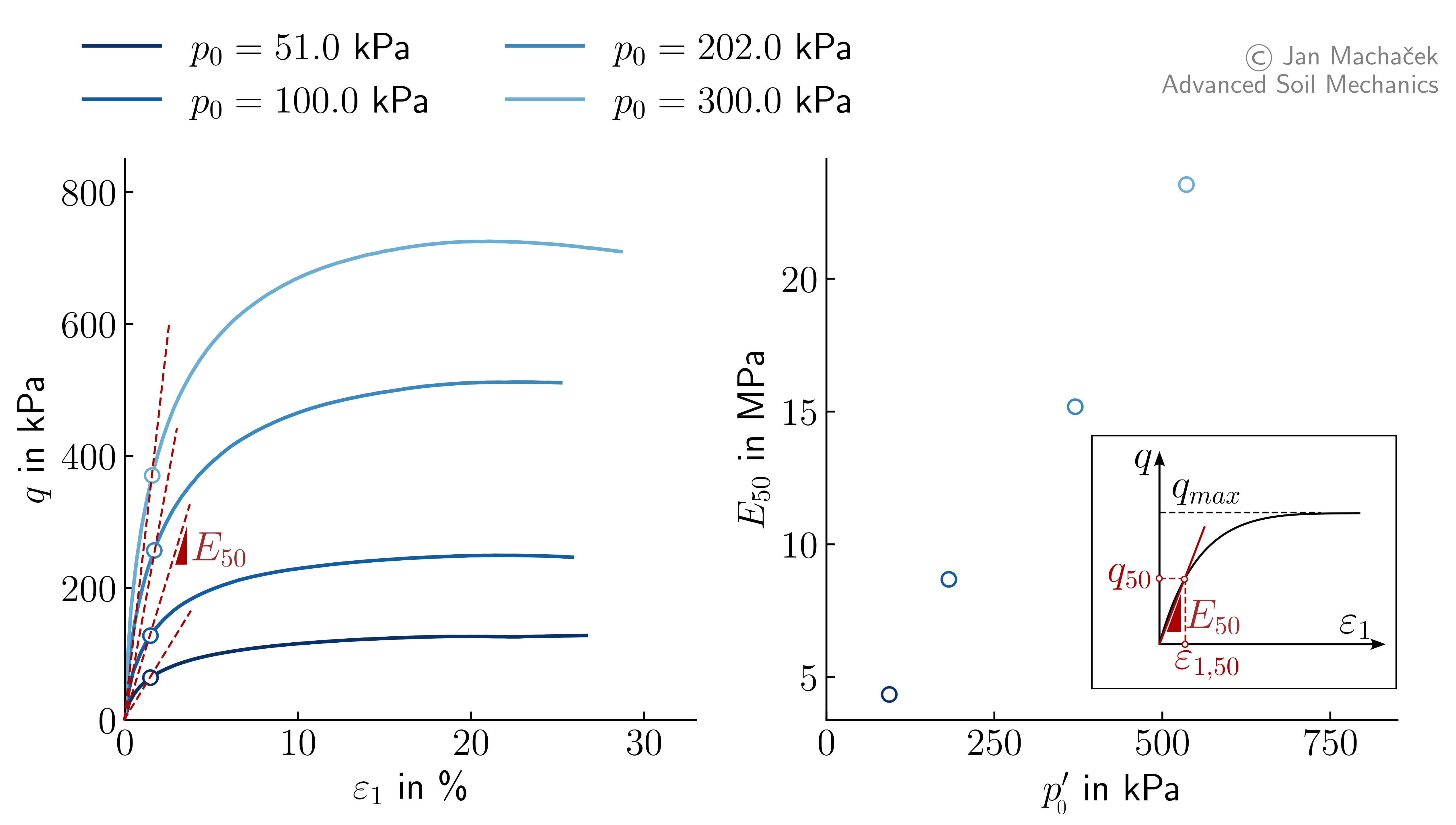
Figure 4. Drained triaxial compression tests on samples of loose Karlsruhe Finesand with different initial mean effective stresses \(p_0^\prime\).

The influence of the stress ratio was also observed in the results of drained and undrained triaxial tests, where the deviatoric stress \(q\) was increased starting from an isotropic stress state (\(q=0\)). Here we observed that the soil samples show large strains for small stress changes at stress ratios close to the critical stress ratio - the stiffness of soils decreases for stress states close to the critical state.

Void ratio dependency and Dilatancy

Similar to the stress state, the void ratio (or density) influences the stiffness of soils. This is illustrated by evaluating \(E_{50}\) for three drained monotonic triaxial tests with different initial relative densities but identical initial mean effective stress \(p_0^\prime=50\) kPa. The results are displayed in Figure 5.

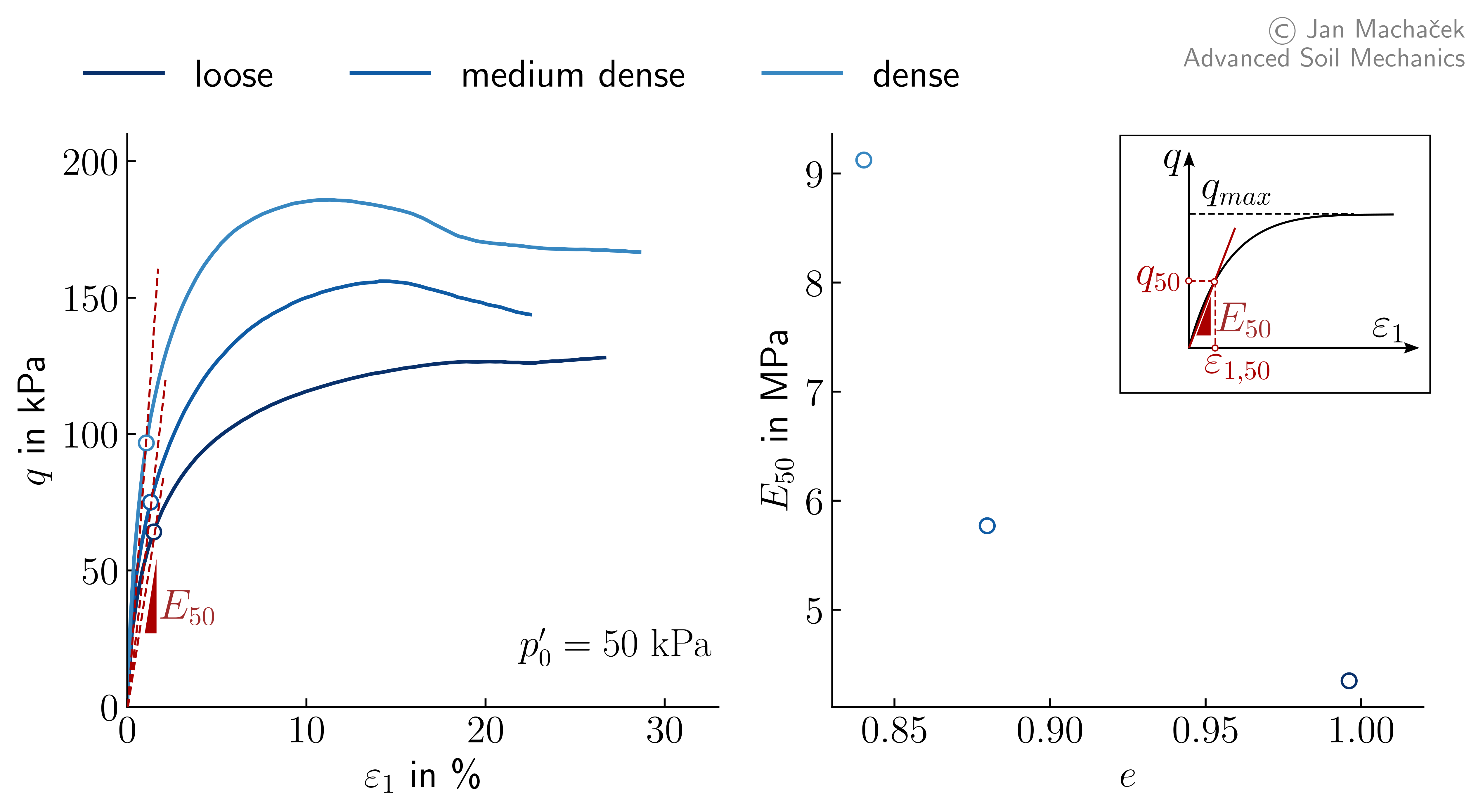
Figure 5. Drained triaxial compression tests on samples of Karlsruhe Finesand with different initial relative densities but identical initial mean effective stress \(p_0^\prime=50\) kPa.

It can be seen that with decreasing void ratio, thus increasing density, the stiffness of soils (sand in this case) increase. Similar observations are made for cohesive soils. In the latter case, this dependency is sometimes reported in terms of the over-consolidation ratio OCR. With increasing OCR the stiffness of cohesive soils increase. An increase in OCR is analogous to a decrease in void ratio.

The influence of the void ratio on soil behaviour is often referred to as Pyknotropy. It plays a crucial role for the state-dependent description of the soil behaviour and has been established as a state variable practically in all advanced constitutive models.

In addition to the influence on the stiffness of soils, the void ratio is an important parameter for describing the dilatancy behaviour of soils. The dilatancy D expresses the maximum rate of volume increase during shear:

\[ D = \dfrac{\dot{\varepsilon}_v}{\dot{\varepsilon}_q} \]

By increasing the relative soil density and thus reducing the void ratio, the maximum shear strength and also the dilatancy increase. This is shown in Figure 6 (right) by means of results from triaxial compression tests on loose and dense sand samples. However, the soil condition changes during deformation and is in fact pressure-dependent. This means that a "dense" soil at a low mean pressure can behave like a loose soil at a high mean pressure. Many models rely on the distance of the void ratio to the critical state \(e_c(p)\) as a measure of density and thus the expected degree of dilatancy. An example for such a measure is the state parameter \(\psi=e-e_c\) shown in Figure 6 (left) and introduced in Chapter Critical State Soil Mechanics.

Figure 6. Left: Concept of the state parameter \(\psi\) as a measure for soil density and expected dilatancy behaviour. Middle and Right: Drained monotonic triaxial tests on dense and loose sand.

Strain dependece

As already discussed in Section Basics of Soil Dynamics, the stiffness of soils also depends on the magnitude of strain. This dependency is qualitatively shown in Figure 7 for the shear modulus \(G\). At small strains, soil stiffness is high and it decays to a lower value as strains increase. The rate of decay is particularly high in the typical ranges of strain occurring around geotechnical structures.

Figure 7. Qualitative dependence of the shear modulus \(G\) on the shear strain \(\gamma\).

Strain should not be a state variable

Note that the strain tensor should not be considered as a state variable since soils do not possess a unique reference configuration in which strain corresponds to zero.

Limit state

Similar to other materials, the stresses or stress states that soils can withstand are inherently limited. This implies the existence of 'compatible' stress states, which can be induced by external loads and absorbed by the soil without leading to failure, and 'incompatible' stress states, which the soil cannot sustain. When subjected to incompatible stress states, soils undergo rearrangement processes within their grain or aggregate structures. This results in a redistribution of stress as the soil effectively 'evades' the applied load.

Such rearrangement processes are characterized by increasing deformations and continue until a compatible stress state is achieved. Hence, there exists a distinct boundary, called limit state, differentiating between compatible and incompatible stress states. This limit stress state is characterised by vanishing stiffness, i. e., \(\dot{\sigma}^\prime=0\). However, it is important that no unique limit stress state exists for soils due to the state dependence of soil behavior. The magnitude of the limit stress depends on the magnitude of deformation and the state of the soil (e.g. stress state, density) as illustrated in Figure 8.

Figure 8. Left: Qualitative dependence of the limit state on density and strain. Middle: Shape of the limit state in principal stress space based on experimental data from Lade (1997). Right: Different mathematical models to describe the limit stress state.

In Chapter Triaxial tests we observed that during triaxial compression and triaxial extension the limit shear stress \(q_f\) at failure could be described by a straight line in the \(q-p^\prime\) plane:

\[ q_{f} = M_{c/e} p^\prime ~~~ \text{where:} ~~~ M_c = \dfrac{6 \sin{\varphi_c}}{3-\sin{\varphi_c}} ~~~\text{and}~~~ M_e = \dfrac{6\sin{\varphi_c}}{3-\sin{\varphi_c}} \]

Therein, \(M_c\) and \(M_e\) are the slopes of the limit state under triaxial compression and triaxial extension, respectively. These, however, are very specific stress paths. In real-case loading scenarios stress paths (and stress ratios) different from triaxial compression and triaxial extension will occur. The effect of such stress path on the limit stress state was investigated for example by Lade (1977)³ by performing true triaxial tests (\(\sigma^\prime_1\), \(\sigma^\prime_2\) and \(\sigma^\prime_3\) can be controlled independently) on Monterey Sand. The result of this study is presented in Figure 7 (middle) showing the shape of limit stress state in principal stress space. It should be noted, that experiments on clay (e.g. Lade & Musante (1978)⁴) show similar shapes for the limit stress state.

A range of theoretical and empirical models propose various shapes for the mathematical approximation of the limit stress surface in the deviatoric plane, as shown in Figure 8 (right).

Advanced features

The list of features discussed so far concentrates on very basic aspects of soil behaviour. The very different structure of soils (compare sand and clay) leads to sometimes very different behavior under load. The basic properties mentioned at the beginning are to be understood as the minimum requirements for material models, which are necessary for a numerical description of the stress-strain behavior of soils. Many properties, including those that you have already encountered in the course of this lecture, are not included in this list. Examples of this are (not exhaustive):

Anisotropy: Most soils are anisotropic to some extent. Anisotropy in strength and stiffness of soils can for example originate from the fabric of soils (reflecting the deformation history) or from stress and strain changes. The former is usually referred to as inherent anisotropy, while the latter is referred to as induced anisotropy. Properties of anisotropic materials depend on the orientation with reference to the coordinate system.
Creep and Viscosity. Creep (or secondary compression) is deformation that continues even after excess pore pressures have dissipated and under constant pore pressure and effective stress. Alternatively, if deformations are constrained, stress relaxation will occur over time. It is a major contributor to the deformation of soft clays, silts and peat. Often it is assumed that stress–strain behaviour is independent of strain rate. However, in Section Observations (Clay, remoulded) we have observed the influence of the strain rate on the material response, the so-called viscosity, based on experiments on a Kaolin with a plasticity index of \(I_p = 12\) %: with increasing strain rate the deformation behaviour was less contractive behaviour and the undrained shear strength moderately increased. In general, stronger strain rate effects are expected for materials with higher plasticity.
Partial saturation. If the soil is not fully saturated, it must be considered as a three-phase material. The definition of the effective stress becomes less obvious. An additional stress variable, mostly the suction as a difference between air and water pressure, is needed in order to model the observed phenomena such as the increase in shear strength with increasing suction. The latter effect is discussed in Section Shear strength of partially saturated soil.
Cyclic loading and Small strain stiffness

A. Niemunis and C. Karcher, Theoretische Bodenmechanik mit Mathematica. 2022. ↩
I. Herle, Fundamentals of constitutive modelling for soils, ALERT Doctoral School, 2022 ↩
P. V. Lade, ‘Modelling the strengths of engineering materials in three dimensions’, Mechanics of Cohesive-frictional Materials, vol. 2, no. 4, pp. 339–356, 1997, doi: https://doi.org/10.1002/(SICI)1099-1484(199710)2:4<339::AID-CFM36>3.0.CO;2-R. ↩
P. V. Lade and H. M. Musante, ‘Three-Dimensional Behavior of Remolded Clay’, J. Geotech. Engrg. Div., vol. 104, no. 2, pp. 193–209, Feb. 1978, doi: 10.1061/AJGEB6.0000581. ↩