Newton-Raphson method

We recall that after discretisation and integration of the balance of linear momentum the resulting system of equations reads

\[ \mathbf{M}\ddot{\mathbf{u}}^* - \mathbf{F}^{int}(\mathbf{u}^*) - \mathbf{F}^{ext} \approx \mathbf{R}(\mathbf{u}^*) \]

stating that the sum of the inertia forces \(\mathbf{M}\ddot{\mathbf{u}}^*\), internal \(\mathbf{F}^{int}(\mathbf{u}^*)\) and external \(\mathbf{F}^{ext}\) forces should be zero for the system to be in equilibrium. Due to the approximated nature of the discretisation and numerical integration this equation can not be fulfilled exactly anymore leading to the existence of a residuum \(\mathbf{R}(\mathbf{u}^*)\). The objective is now to find \(\mathbf{u}^*\) such that the system is in equilibrium, i.e. \(\mathbf{R}(\mathbf{u}^*)\) becomes close to zero.

Since the system of equations is (strongly) non-linear in the general case, and in geotechnics in particular, a direct solution is usually not possible. The non-linearities can come, for example, from the stress- and density-dependent stiffness of the soil or the soil-structure interaction. A widely used method for solving such non-linear equations is the Newton-Raphson method, which was proposed by Newton in 1669 and generalised by Raphson in 1690. The procedure is first explained for a system with only a single degree of freedom neglecting inertia effects:

\[ \begin{equation}\label{eq:newton-raphson-general} F^{int}(u^*) - F^{ext} \approx R(u^*) \end{equation} \]

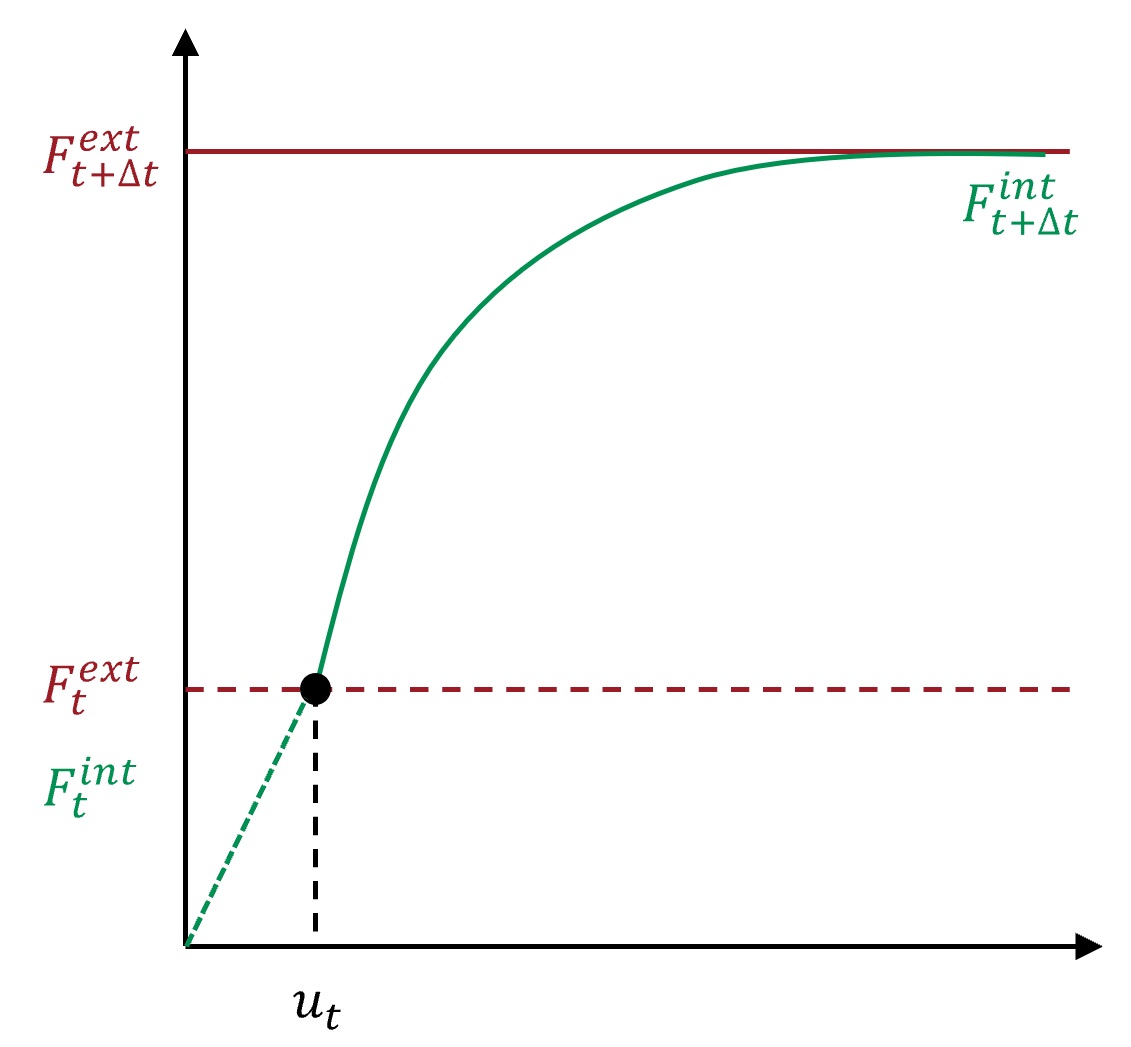
The solution of this equation at time \(t\) is known, the solution at time t + delta t is sought. More precisely: for a given external load \(F^{ext}_{t+\Delta t}\) at time \(t+\Delta t\), the displacement \(u^*_{t+\Delta t}\) is sought so that the system is in equilibrium, i.e. \(F^{ext}_{t+\Delta t} \approx F^{int}_{t+\Delta t}(u^*)\). A schematic diagram of the solution is shown below

It is assumed that the solution to Equation (\(\ref{eq:newton-raphson-general}\)) is continuous allowing to perform a Taylor series expansion to approximate the solution to \(R(u^*)\):

\[ R(u^*)^{i+1} \approx R(u^*)^{i} + \dfrac{\partial R(u^{*,i})^{i}}{\partial u^*} \left( u^{*,i+1}-u^{*,i} \right) + \dfrac{1}{2!}\dfrac{\partial^2 R(u^{*,i})^{i}}{\partial (u^*)^2} \left( u^{*,i+1}-u^{*,i} \right)^2 + ... \]

Neglecting higher-order terms we obtain:

\[ R(u^*)^{i+1} \approx R(u^*)^{i} + \dfrac{\partial R(u^{*,i})^{i}}{\partial u^*} c^{*,i+1} ~~~{\text{with:}~~~ } c^{*,i+1} = u^{*,i+1}-u^{*,i} \]

Since we are aiming to find \(u^{*,i+1}\) such that \(R(u^*)^{i+1}\) vanishes, we set \(R(u^*)^{i+1}=0\) and rearrange above equation:

\[ \dfrac{\partial R(u^{*,i})^{i}}{\partial u^*} c^{*,i+1} = - R(u^*)^{i} \]