Elasticity
In elasticity, a linear or non-linear relationship between stress and strain is assumed in which the deformations are completely reversible, i.e. no plastic deformations occur. This is illustrated in Figure 1.
For soils, however, plastic and cumulative deformations can only be neglected for very small strain amplitudes of \(\sim10^{-5}\) for sand and \(\sim 10^{-4}\) for clay1. The range of validity of elastic models in geotechnical engineering is therefore strictly limited to the range of very small deformations. Because of these limitations, elasticity in geotechnics is mainly used to calculate wave propagation. However, it is an integral part of elasto-plastic models, as we will see in the following sections, and therefore deserves special attention.
Types of elasticity
In general, elastic models can be divided into three classes:
-
Cauchy elasticity (or simple elasticity)
A stress-strain relationship is Cauchy-elastic or simple elastic if a one-to-one relationship between stress and strain exists, or in other words, when stress is determined only by the current strain:
\[ \sigma_{ij} = f_{ij}(\varepsilon_{kl}) \]The function \(f_{ij}\) is a smooth tensor-valued function and often called "response function". A one-to-one relationship also means that the strain can be determined from the inverse of this relationship:
\[ \varepsilon_{kl} = f_{kl}^{-1}(\sigma_{ij}) \] -
Hypo-elasticity
In Hypo-elasticity an incremental but still reversible stress-strain relationship is used:
\[ \dot{\sigma}_{ij} = E_{ijkl} \dot{\varepsilon}_{kl} \]The relationship can be path/state-dependent, i.e. \(E_{ijkl}\) is allowed to change. An example from geotechnical engineering of a hypo-elastic model would be to consider the stress dependence of stiffness in the following form (given in 1D for the sake of simplicity)
\[ \dot{\sigma} = E_{ref} \left( \dfrac{\sigma}{\sigma_{ref}} \right)^{n_\sigma} \dot{\varepsilon} \]where \(E_{ref}\) is a reference stiffness evaluated at a given reference pressure \(\sigma_{ref}\) and the exponent \(n_\sigma\) controls the increase of stiffness with increasing effective stress.
-
Hyper-elasticity
Hyper-elasticity is also known as Green's elasticity or true elasticity. In contrast to cauchy- or hypo-elasticity, the stress is calculated from the strain energy density (or elastic potential) \(W(\varepsilon_{ij})\)
\[ \sigma_{ij} = \dfrac{\partial W}{\partial \varepsilon_{ij}} \]The unit strain density function (or elastic potential) \(W\) describes the strain energy per unit volume as a function of a general strain state \(\varepsilon_{ij}^t\) at time \(t\):
\[ W(\varepsilon_{ij}^t) = \int_0^{\varepsilon_{ij}^t} \sigma_{ij} \text{d} \varepsilon_{ij} \]Alternatively hyper-elastic constitutive models can also be formulated in terms of the complementary energy density \(\bar{W}(\sigma_{ij})\):
\[ \varepsilon_{ij} = \dfrac{\partial \bar{W}}{\partial \sigma_{ij}} \]where the complementary energy density \(\bar{W}(\sigma_{ij})\) describes the energy per unit volume as a function of the stress state and is defined as follows:
\[ \bar{W}(\sigma_{ij}) = \sigma_{ij} \varepsilon_{ij} - W(\varepsilon_{ij}) \]A graphical representation of \(W(\varepsilon_{ij})\) and \(\bar{W}(\sigma_{ij})\) is given in Figure 2.
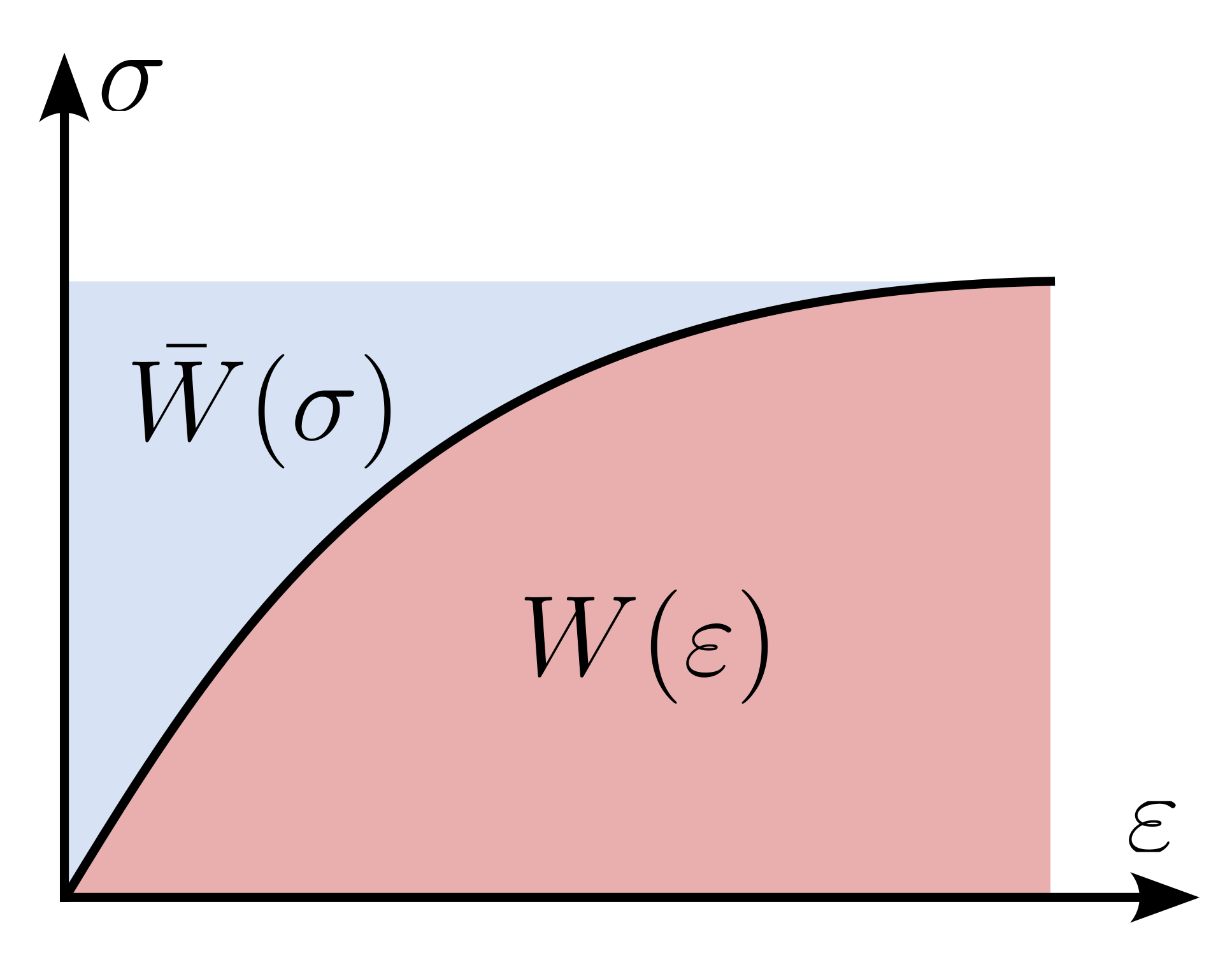
Figure 2. Schematic representation of the strain density function \(W(\varepsilon_{ij})\) and the complementary energy density \(\bar{W}(\sigma_{ij})\).Finding an elastic potential \(W(\varepsilon_{ij})\) and \(\bar{W}(\sigma_{ij})\) that yields a useful elastic stress-strain relation or stiffness \(E_{ijkl}\) for soil mechanics is a difficult task1. The tangent stiffness is defined as \(E_{ijkl}=\partial \sigma_{ij}/ \partial \varepsilon_{kl}\) and thus reads:
\[ E_{ijkl} = \dfrac{\partial^2 W}{\partial \varepsilon_{ij} \partial \varepsilon_{kl} } \]
It is worth noting that a hypo-elastic model can be hyper-elastic or cauchy-elastic, depending on its formulation. Similar, a hyper-elastic model can be cauchy-elastic. An example for the latter case is the isotropic linear elasticity. Although all models are elastic, they differ in terms of their formulation and energy conservation characteristics. Consideration of a closed strain path (i.e. the starting point and the end point of the strain path are identical) as shown in Figure 3
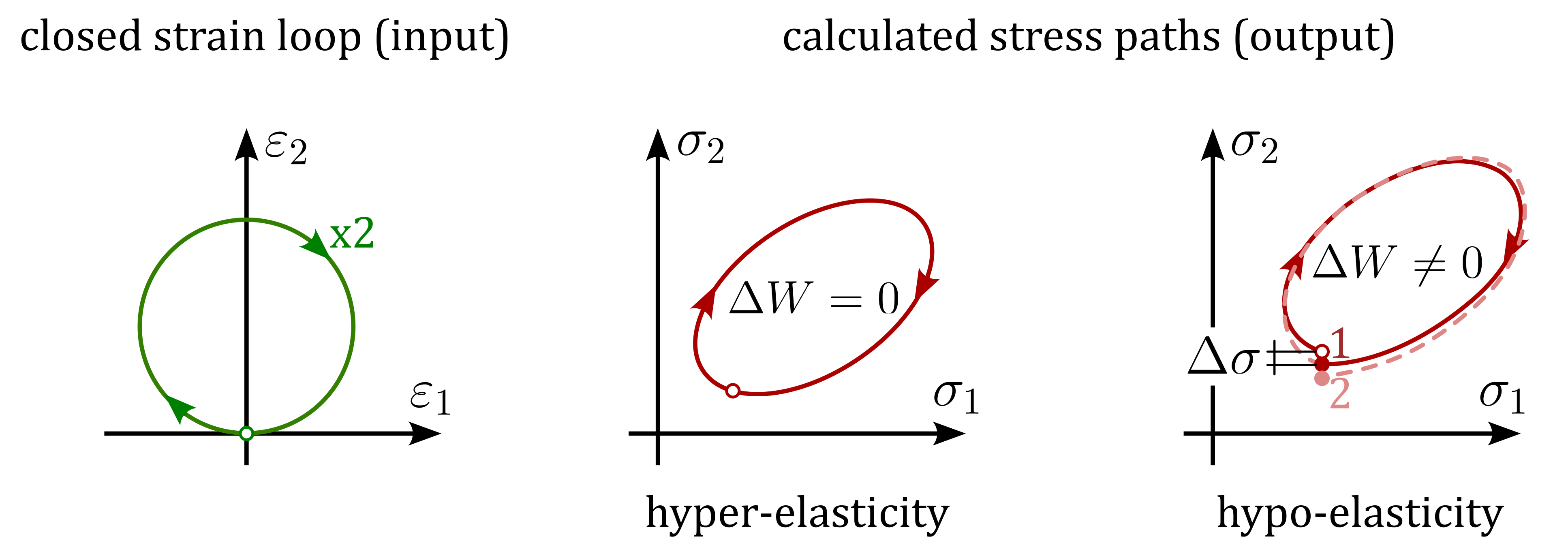
Figure 3. Calculated stress paths for a prescribed closed strain paths with two cycles. For a hypo-elastic material model, a closed strain path can result in an accumulation of stress (\(\Delta \sigma \neq 0\)) and a dissipation of energy (\(\Delta W \neq 0\))
shows that:
-
In the case of hyper-elasticity a closed stress path follows from a closed strain path. No dissipation of energy is observed (\(\Delta W = 0\)). The reason for this is, that the deformation work is independent of the path, which is expressed in the fact that the deformation work only depends on the start and end points of the deformation path, but not on its path.
-
For hypo-elasticity, e.g. for barotropic (stress-dependent) elasticity, energy conservation cannot be guaranteed. A closed strain path may lead to an open stress path, thus accumulation of stress \(\Delta \sigma \neq 0\). In such cases, dissipation of energy occurs (\(\Delta W \neq 0\)). The reason for the accumulation of stress is the path dependency of the model as shown in Figure 3 for the example of a barotropic elasticity.
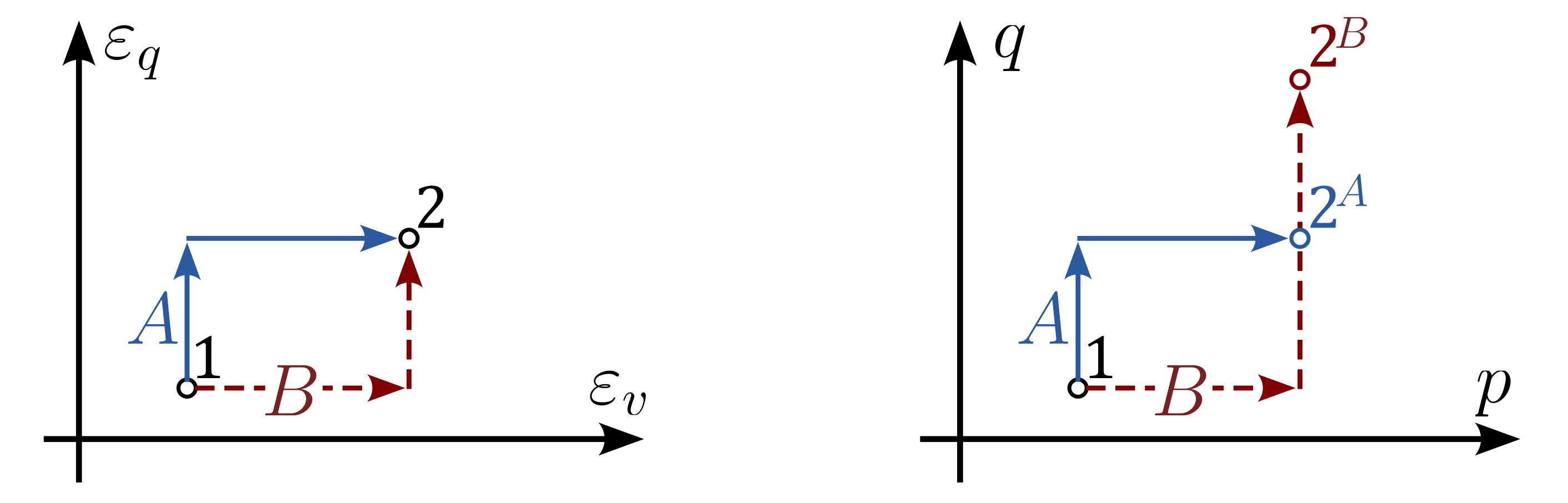
Figure 4. Path dependency of stress dependent (barotropic) hypo-elastic material. Modified from Niemunis (2014)2In the case of cyclic loading, this can lead to an unintended accumulation of deformation or stress. The direction of accumulation depends on the direction in which the expansion path is traversed (clockwise or anti-clockwise).
For cyclic loading, eg. the calculation of a wave propagation, the use of hypo-elastic models is strongly discouraged and hyper-elastic models are recommended.
Isotropic linear elasticity
Isotropic linear elasticity is a special case of hyper-elasticity. Due to the underlying assumption of constant stiffness, i.e \(E_{ijkl} = const\), it also satisfies the condition of Cauchy elasticity \(\sigma_{ij} = f_{ij}(\varepsilon_{kl})\):
The corresponding elastic potential (stress energy function) reads
In geotechnical engineering, isotropic linear elasticity is mainly used to simulate wave propagation and as the "elastic component" of simple elasto-plastic constitutive models such as the Mohr-Coulomb model. The stiffness tensor \(E_{ijkl}\) is defined as
Therein, the Young's modulus \(E\) and the Poisson's ratio \(\nu\) are constants. \(G\) is the shear modulus. The isotropic linear elastic model thus has only two parameters. Another frequently encountered notation uses the Lamé constants \(\lambda = \frac{E \nu}{(1+\nu)(1-2\nu)}\) and \(\mu = G\):
With above definition of the stiffness tensor, the stress rate reads in index notation
The above equation shows that deviatoric and volumetric components of the isotropic linear stiffness can be considered separately. This means that
-
From purely volumetric strain \(\dot{\varepsilon}_{kl} = \delta_{kl} \dfrac{1}{3} \dot{\varepsilon}_{vol}\) only changes in hydrostatic stress (pressure) result:
\[ \dot{\sigma}_{ij} = \left( \lambda \delta_{ij} \delta_{kl} + 2 \mu I_{ijkl} \right) \delta_{kl} \dfrac{1}{3} \dot{\varepsilon}_{vol} = \delta_{ij} \left( \lambda + 2 \mu \right) \dfrac{1}{3} \dot{\varepsilon}_{vol} \]with the definition of the mean stress \(p=\dfrac{1}{3} \delta_{ij} \sigma_{ij}\) introduced in section Roscoe invariants the rate of mean stress \(\dot{p}\) reads
\[ \dot{p} = \dfrac{1}{3} \delta_{ij} \dot{\sigma}_{ij} = \left( \lambda + 2 \mu \right) \dot{\varepsilon}_{vol} = K \dot{\varepsilon}_{vol} \]where \(K = \left( \lambda + 2 \mu \right) = \dfrac{E}{3(1-2\nu)}\) is called the bulk modulus.
-
Purely deviatoric strain \(\varepsilon_{kl}^*\), only result in changes in deviatoric stresses \(\sigma_{ij}^*\)
\[ \dot{\sigma}_{ij} = \left( \lambda \delta_{ij} \delta_{kl} + 2 \mu I_{ijkl} \right) \varepsilon_{kl}^* = 2 \mu \varepsilon_{ij}^* = 2 G \varepsilon_{ij}^* = \dot{\sigma}_{ij}^* \]
With above considerations we can come to an alternative equation for the stress rate in terms of the bulk modulus \(K\) and the shear modulus \(G\):
Parameter calibration
The isotropic linear elastic constitutive model has two parameters:
- Young's modulus \(E\): relationship between stress and strain
- Poisson ratio \(\nu\): measure for the deformation of a material in directions perpendicular to the specific direction of loading.
In geotechnics the shear modulus \(G\), the bulk modulus \(K\) and the constrained modulus \(M\) are widely used quantities. They are related to \(E\) and \(\nu\) as follows:
The fact that the isotropic linear elastic model has only two parameters leads on the one hand to a supposedly simple calibration of the model, but also to a limited flexibility of the model to adapt to the real observed behaviour of soils. It is obvious that the model does not take into account almost all the required properties of a material model for soils presented in Section Features of constitutive models for soils. For example, the model does not satisfy the requirement of non-linearity (e.g. due to the pressure and void ratio dependence of the material), the stress-strain paths are fully reversible (violates the requirement of irreversibility) and the model does not consider limit states.
The calibration of the model is particularly affected by the lack of consideration of stress and void ratio dependence, which means that (strictly speaking) the material behaviour can only be calibrated for a single stress state and density. This is demonstrated below using an oedometric compression test and a series of triaxial tests.
Large strains
For the application of the isotropic linear elastic model to large deformations such as settlement calculations or as part of a simple elasto-plastic model, the Young's modulus is usually determined based on results of oedometric compression tests or triaxial compression tests.
If the results of an oedmoetric compression test are plotted in terms of the vertical (or axial) strain \(\varepsilon_v\) over the vertical (or axial) stress \(\sigma_v\), the stiffness can directly be determined from the inclination of the stress-strain path:
\(M\) is the constrained modulus. The Young's modulus \(E\) cannot be determined directly from an oedometric compression test due to its inherent boundary conditions (no permitted horizontal/radial deformation), but can be determined from \(M\) if the Poisson's ratio \(\nu\) is known (see above). The results of an oedometric compression test on sand are displayed in Figure 5.
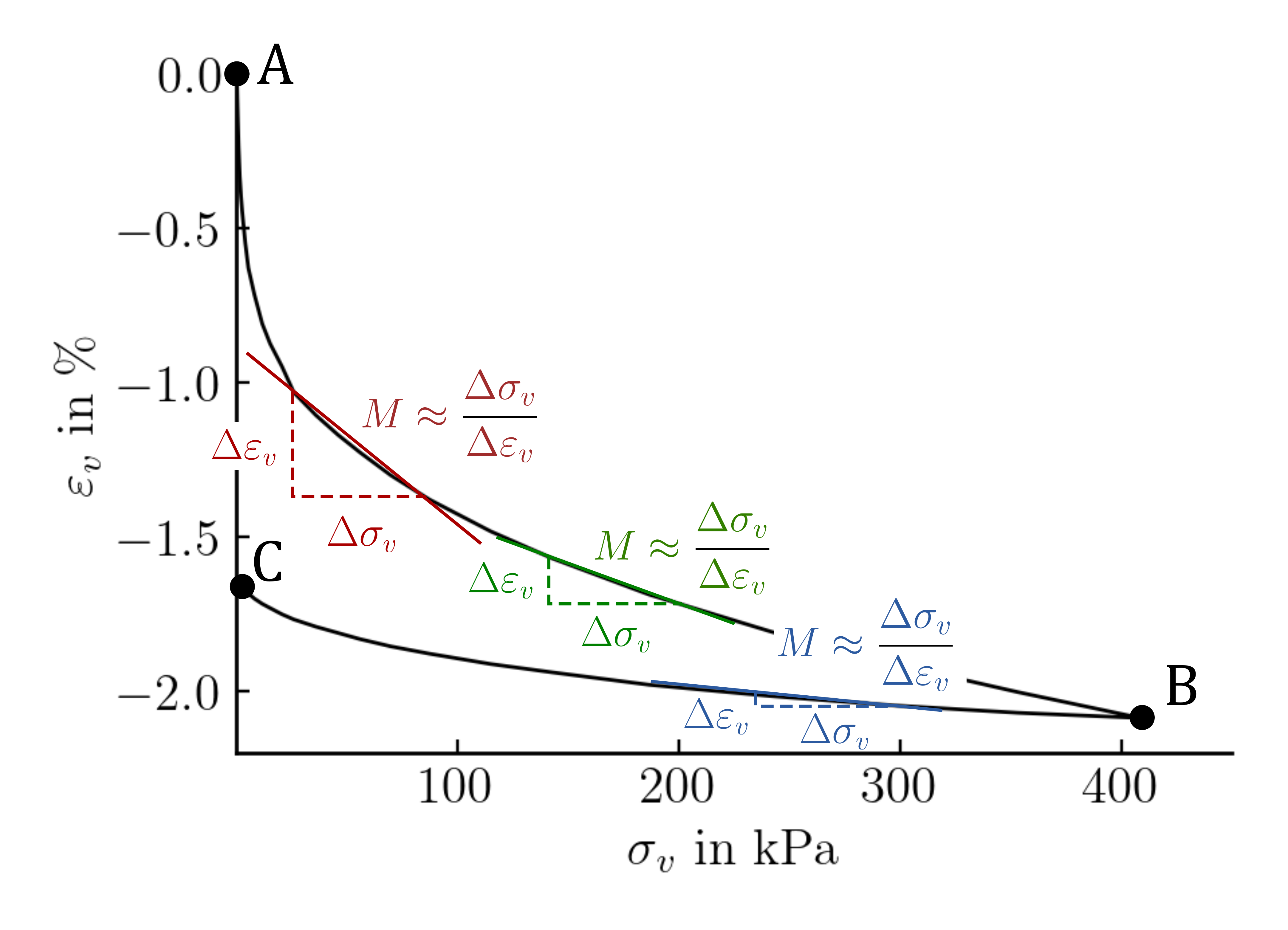
Figure 5. Oedometric compression test on sand with loading and unloading.
It is obvious, that the ratio \(\dot{\sigma}_v/\dot{\varepsilon}_v\) is not constant but changes not only during loading and unloading but also significantly during the (primary) loading part of the experiment. It is thus common to evaluate \(M\) as a linear approximation for a given stress or strain increment:
From Figure 5 it also becomes obvious that changes in \(M\) are more pronounced during the loading path A-B of the experiment. Contrary, during an unloading path \(B-C\), changes in \(M\) are less pronounced rendering the assumption of a linear elastic behaviour during unloading \(M^{A-B}=const\) a reasonable simplification.
Alternatively, the Young's modulus \(E\) can be determined based on the results of drained triaxial compression tests. Usually this is done in terms of the secant stiffness evaluated at 50% of the maximum deviatoric stress \(q_{50} = q_{max}/2\):
where \(\varepsilon_{1,50}\) is the axial strain corresponding to \(q_{50}\). Although easy to evaluate, \(E_{50}\) should in fact not be a constant as it changes with mean (effective) stress and void ratio as discussed in Stress dependence and Void ratio dependency. This is demonstrated by evaluating \(E_{50}\) on results from a series of drained monotonic triaxial tests with different initial mean effective stresses \(p_0^\prime\) summarized in Figure 6.
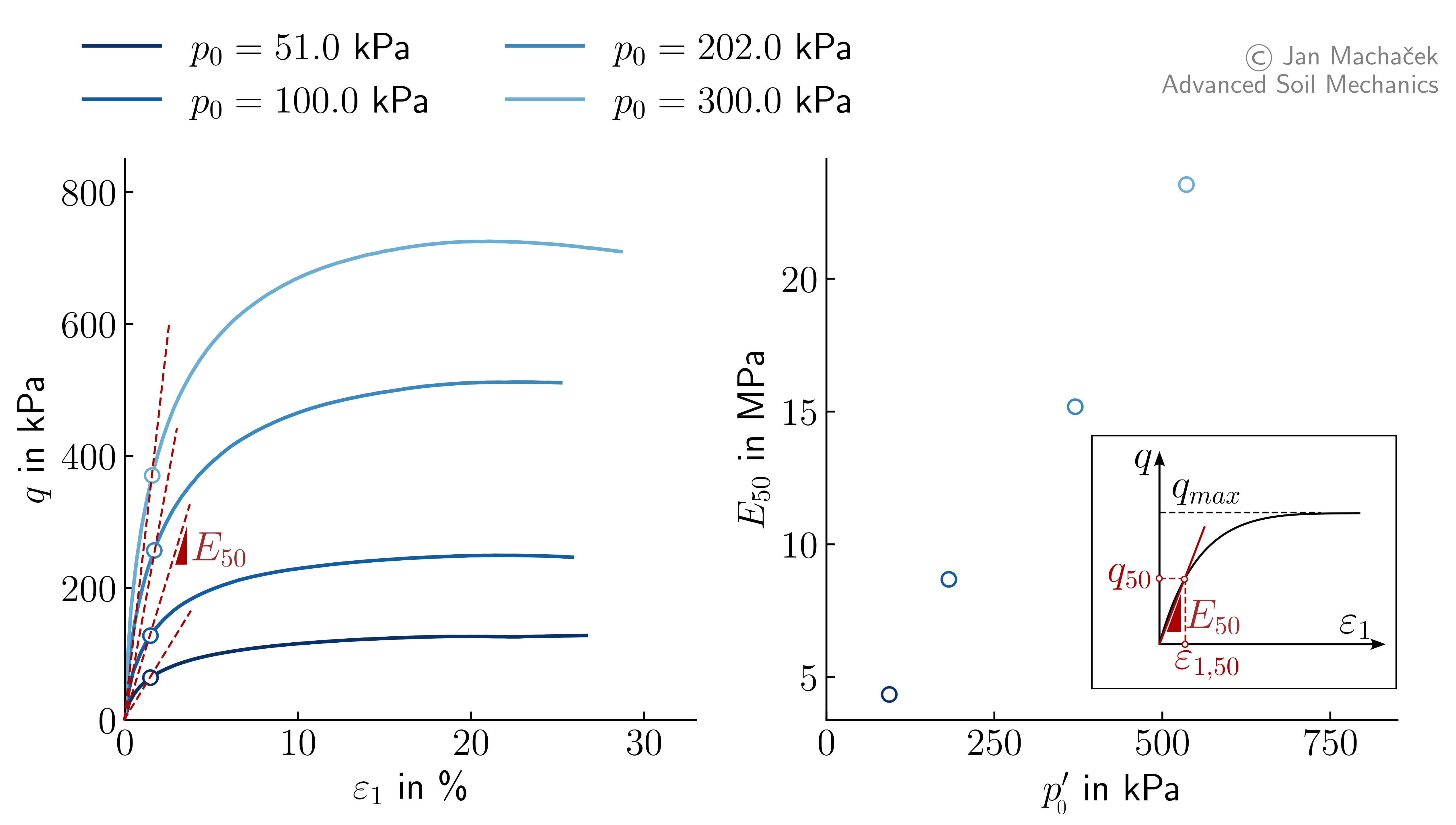
Figure 6. Drained triaxial compression tests on samples of loose Karlsruhe Finesand with different initial mean effective stresses \(p_0^\prime\).
The Poisson's ratio \(\nu\) can be determined from triaxial compression tests as the ratio of the radial strain rate to the axial strain rate, i.e. \(\nu = \dot{\varepsilon}_r/\dot{\varepsilon}_1\). However, the radial strain \(\varepsilon_r\) is usually not measured in triaxial compression tests. From the definition of the volumetric strain rate \(\dot{\varepsilon}_v = \dot{\varepsilon}_1 + 2\dot{\varepsilon}_r\) (see Triaxial test) it follows that:
Determining \(\nu\) based on standard oedometric compression tests is not possible as the horizontal/radial stresses \(\sigma_r\) during the test are unknown. Special oedmoetric compression tests, known as soft oedometer, measuring the radial stresses during the experiment are required. If the radial and axial stresses (\(\sigma_r\) and \(\sigma_a\)) are known, the Poisson ratio can be calculated from
Small strains
For small strains, e.g. the simulation of wave propagation, the elastic constants \(G\), \(K\) and \(\nu\) can be determined from measured wave velocities:
where \(\rho\) is the density of the soil, \(c_s\) and \(c_p\) are the shear wave and compression wave velocities, respectively. The Young's modulus \(E\) can then be calculated from \(G\) and \(\nu\) or \(K\) and \(\nu\). More details are given in Chapter Basics of Soil Dynamics – soil behaviour under dynamic loading / at (very) small strains.