Notation

The notation and terminology used throughout this course are explained below. Internalizing these is essential for understanding the covered content. In particular, distinguishing between scalars, vectors, and tensors, as well as the mathematical handling of these, is of great importance.

Scalars

A scalar represents a quantity without a directional component, and its value remains unchanged regardless of the coordinate system. Examples include mass \(m\) or time \(t\). Throughout this course, scalars are written in normal font, e.g. \(a\).

Vectors

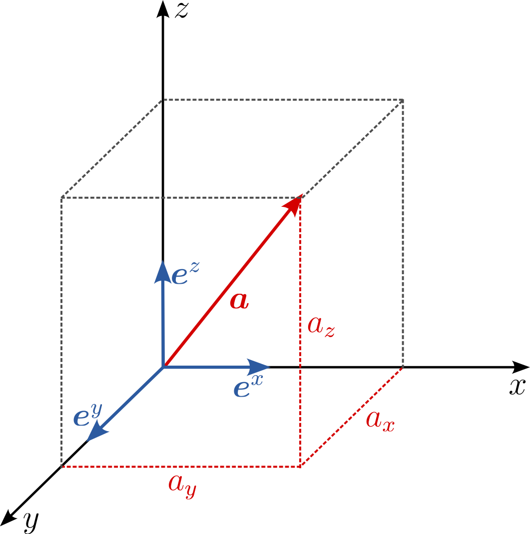
A vector, in its most general sense, consists of an ordered set of values called 'vector components'. In 3-D space specifically, there are three such values. Combined with directional indicators \(\mathbf{e}^i\), or 'basis vectors', they define a geometric entity. However, it's important to note that vectors can exist in spaces of any dimension, not just 3-D. The vector's magnitude remains invariant (meaning it doesn't change), even if its components might differ based on the chosen coordinate system. Common examples of vectors include displacement and velocity. Vectors are typically represented in a bold lowercase font, e.g. \(\boldsymbol{a}\), or using index notation as \(a_i\), where the index \(i\) refers to a specific component of the vector (e.g., \(i=1\) might correspond to the \(x\)-component, \(i=2\) to the \(y\)-component, and \(i=3\) to the \(z\)-component in a 3-D space).

Tensors

A tensor provides a mathematical representation of a more general physical or geometric concept that might be characterized by both magnitude and multiple directions. In 3-D space, a tensor of rank \(n\) (or an nth-order tensor) has \(3^n\) components. These components, when associated with multiple directional indicators known as 'basis vectors', define an entity that transforms in a specific manner when the coordinate system is changed. It's this transformation behavior that distinguishes tensors from other mathematical entities. A classic example in the context of solid mechanics is the stress tensor, which represents the internal forces in a material and has nine components in 3-D space. This tensor provides information about magnitudes and directions, capturing the complex state of stress within a material. A graphical interpretation of tensors of different ranks is provided below (modified from²)

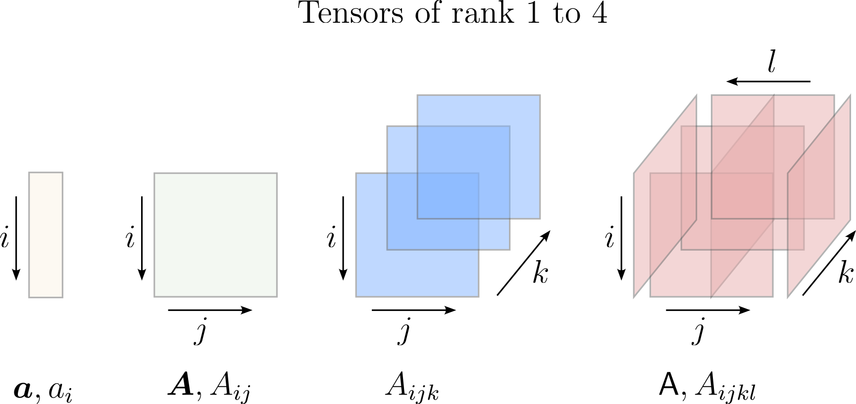
Graphical interpretation of tensors of different ranks

Second order tensors are usually written in uppercase or Greek symbol bold font, e.g., \(\mathbf{A}\) or using index notation as \(A_{ij}\). Here, the indices \(i\) and \(j\) each refer to a specific component direction of the tensor (e.g., \(i=1, j=1\) might correspond to the \(x\)-direction stress on a face perpendicular to the \(x\)-direction, and so on). Another representation, although less common and not in use in this class, is \(\underline{A}\). An example of a second-order tensor is the aforementioned stress tensor:

\[ \boldsymbol{\sigma} = \begin{bmatrix} \sigma_{xx} & \sigma_{xy} & \sigma_{xz} \\ \sigma_{yx} & \sigma_{yy} & \sigma_{yz} \\ \sigma_{zx} & \sigma_{zy} & \sigma_{zz} \end{bmatrix} \]

Index notation

Index notation, often referred to as the Einstein summation convention, originated in the early 20th century and was popularized by Albert Einstein. It provides a concise way to represent long and complex mathematical operations, particularly in the realms of vectors and tensors.

A vector \(\boldsymbol{a}\) is expressed in index notation as

\[ (\boldsymbol{a})_{i}=a_i. \]

Likewise, a second rank tensor is denoted by

\[ (\boldsymbol{M})_{ij} = M_{ij}. \]

The operations

\[ ()_i ~~~\text{and}~~~ ()_{ij} \]

are used to extract the \(i\)th component of a vector and the \(ij\)th component of a tensor, respectively. It is imperative to note that a mixed notation such as \(\boldsymbol{M} = M_{ij}\) is formally incorrect because the left side represents the tensor itself, while the right side denotes one of its components¹.

Why index notation?

Index notation is favored not only for its brevity but also for its precision in describing intricate tensor operations. A key feature of this notation is the convention of summing over repeated indices: a repeated index in a term automatically implies summation over that index. For example, if two variables have the same index, it indicates summation over the range of that index, removing the need for explicit summation symbols.

Basic mathematical operations

For the following examples we restrict ourself to 3 dimensions. Let

\[ \mathbf{a}=\{a_1,a_2,a_3\} ~~~\text{and} ~~~ \mathbf{b}=\{b_1,b_2,b_3\} \]

be vectors of length 3, while \(\mathbf{M}\) and \(\mathbf{T}\) are tensors of rank 2 and size (3x3):

\[ \mathbf{M} = \begin{bmatrix} M_{11} & M_{12} & M_{13} \\ M_{21} & M_{22} & M_{23} \\ M_{31} & M_{32} & M_{33} \end{bmatrix} ~~~\text{and} ~~~ \mathbf{T} = \begin{bmatrix} T_{11} & T_{12} & T_{13} \\ T_{21} & T_{22} & T_{23} \\ T_{31} & T_{32} & T_{33} \end{bmatrix} \]

Scalar product between two vectors

In tensor notation, the scalar product between vectors \(\mathbf{a}=\{a_1,a_2,...a_n\}\) and \(\mathbf{b}=\{b_1,b_2,...,b_n\}\) is:

\[ \mathbf{a} \cdot \mathbf{b} \]

In index notation:

\[ a_i b_i = \sum_{i=1}^n a_i b_i = a_1 b_1 + a_2 b_2 + a_3 b_3 \]

\(i\) is called a dummy index because the sum is independent of the letter used.

Scalar product between a 2nd rank tensor and a vector

Multiplying a second rank tensor \(\mathbf{M}\) by a vector \(\mathbf{a}\) to get vector \(\mathbf{b}\) in tensor notation is:

\[ \mathbf{b} = \mathbf{M} \mathbf{a} \]

In index notation:

\[ b_i = M_{ij} a_j = M_{i1} a_1 + M_{i2} a_2 + M_{i,3} a_3 \]

Here \(i\) is called a free index because it appears once in each summand and \(j\) is a dummy index.

Scalar product between two 2nd rank tensors

Multiplying a second rank tensor \(\mathbf{M}\) by an other second rank tensor \(\mathbf{T}\) results in a scalar \(a\):

\[ a = \mathbf{M} : \mathbf{T} \]

In index notation:

\[ \begin{aligned} a &= M_{ij} T_{ij} \\ &= M_{11} T_{11} + M_{12} T_{12} + M_{13} T_{13} \\ & ~~~~ + M_{21} T_{21} + M_{22} T_{22} + M_{23} T_{23} \\ & ~~~~ + M_{31} T_{31} + M_{32} T_{32} + M_{33} T_{33} \end{aligned} \]

Matrix Multiplication of two 2nd rank tensors

The rule for matrix multiplication of two second-order tensors (i.e., two 3x3 matrices) follows the standard rules of matrix multiplication in linear algebra.

If \(\mathbf{M}\) and \(\mathbf{T}\) are both 3x3 matrices, with \(\mathbf{M}\) having elements \(M_{ij}\) and \(\mathbf{T}\) having elements \(T_{ij}\), the product \(\mathbf{P}\) is defined as:

\[ \mathbf{P} = \mathbf{M} \cdot \mathbf{T} = \sum_{k=1}^3 M_{ik} T_{kj} \]

where \(i\) and \(j\) are free indices referring to the row of \(\mathbf{M}\) and the column of \(\mathbf{T}\), respectively. \(k\) is a dummy index and runs over the elements of the row in \(\mathbf{M}\) and the elements of the column in \(\mathbf{T}\):

\[ P_{ij} = A_{i1}T_{1j} + A_{i2}T_{2j} + A_{i3}T_{3j} \]

or in expanded form:

\[ \begin{aligned} P_{11} &= M_{11}T_{11} + M_{12}T_{21} + A_{13}T_{31}, \\ P_{12} &= M_{11}T_{12} + M_{12}T_{22} + A_{13}T_{32}, \\ P_{13} &= M_{11}T_{13} + M_{12}T_{23} + A_{13}T_{33}, \\ P_{21} &= M_{21}T_{11} + M_{22}T_{21} + A_{23}T_{31}, \\ P_{22} &= M_{21}T_{12} + M_{22}T_{22} + A_{23}T_{32}, \\ P_{23} &= M_{21}T_{13} + M_{22}T_{23} + A_{23}T_{33}, \\ P_{31} &= M_{31}T_{11} + M_{32}T_{21} + A_{33}T_{31}, \\ P_{32} &= M_{31}T_{12} + M_{32}T_{22} + A_{33}T_{32}, \\ P_{33} &= M_{31}T_{13} + M_{32}T_{23} + A_{33}T_{33}. \end{aligned} \]

Trace of a 2nd rank tensor

The trace of a tensor \(\mathbf{M}\) in tensor notation:

\[ \text{tr}(\mathbf{M}) \]

In index notation:

\[ \text{tr}(M_{ij}) = M_{ii} = M_{11} + M_{22} + M_{33} \]

The trace of a 2nd rank tensor can also be written using the Kronecker-Delta \(\delta_{ij}\):

\[ \text{tr}(M_{ij}) = \delta_{ij} M_{ij} = M_{ii} ~~~\text{with:}~~~ \delta_{ij} = \begin{cases} 1 &\text{if } i = j \\ 0 &\text{if } i \neq j \end{cases} \]

Kronecker delta

The Kronecker delta, denoted by \(\delta_{ij}\), serves as an identity in index notation and can be employed to interchange indices in a tensor. When multiplied with a tensor, it swaps a repeated (dummy) index with a free index. For instance:

\[ \begin{aligned} a_{i} \delta_{ij} &= a_{j} \\ A_{ij} \delta_{ij} &= A_{ii} \\ A_{ij} \delta_{ik} &= A_{kj} \end{aligned} \]

Euclidean norm of a vector

The Euclidean norm of vector \(\mathbf{a}\) in tensor notation:

\[ ||\mathbf{a}|| = \sqrt{\mathbf{a} \cdot \mathbf{a}} \]

In index notation:

\[ ||a|| = \sqrt{a_i a_i} = \sqrt{a_1 a_1 + a_2 a_2 + a_3 a_3} \]

Frobenius norm of a tensor (Rank 2)

The Frobenius norm of tensor \(\mathbf{M}\) in tensor notation:

\[ ||\mathbf{M}||_F = \sqrt{\text{tr}(\mathbf{M}^T \mathbf{M})} \]

In index notation:

\[ ||M_{ij}||_F = \sqrt{M_{ij} M_{ij}} \]

Determinant of a 3x3 tensor (Rank 2)

The determinant \(\det()\) of a 3x3 tensor \(\mathbf{M}\) is calculated as follows:

\[ \begin{aligned} \det(\mathbf{M}) = \det(M_{ij}) &= M_{11}(M_{22}M_{33} - M_{23}M_{32}) \\&- M_{12}(M_{21}M_{33} - M_{23}M_{31}) \\&+ M_{13}(M_{21}M_{32} - M_{22}M_{31}) \end{aligned} \]

Additional resources

For those who are still struggling with the world of vectors and tensors, Professor Dan Fleisch, Emeritus from the Department of Physics at Wittenberg University, offers a succinct and lucid introduction in the video below.

Disclaimer: This video is the work of Professor Dan Fleisch and is embedded here for educational purposes. No copyright infringement is intended, and all credits go to the original creator.

---

1. A. Niemunis and C. Karcher, Theoretische Bodenmechanik mit Mathematica. 2022. ↩

2. F. Prada, Presentation: Introduction to Tensor Calculus, Advanced Constitutive Models for Geomaterials (WP44), Ruhr-Universität Bochum, 14th April 2023 ↩