Stress tensor

In the context of granular media, such as soils, stress represents an averaged measure of the contact forces between grains over a representative volume. As such, the intricate details of force chains are captured within a continuous and differentiable stress field, which provides both the magnitude and orientation of the averaged contact forces.

Stress vector and stress tensor

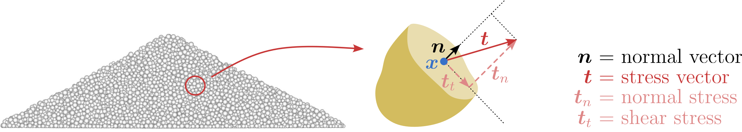
When a body is intersected by a plane in an arbitrary direction, a stress vector \(\boldsymbol{t}(\boldsymbol{x},\boldsymbol{n})\) is freed at any point \(\boldsymbol{x}\) on the resulting cross-section. Both the magnitude and orientation of the stress vector can change based on the orientation \(\boldsymbol{n}\) of the cross-section, where \(\boldsymbol{n}\) represents the normal vector to the cross-section. As depicted in the figure below, the stress vector \(\boldsymbol{t}\) can be decomposed into a normal component \(\boldsymbol{t}_n\) and a tangential component \(\boldsymbol{t}_s\):

\[ \begin{aligned} t_{n_j} &= t_{n_i} n_i n_j \\ t_{t_j} &= t_j - t_{n_j} \end{aligned} \]

The stress tensor \(\boldsymbol{\sigma}(\boldsymbol{x})\) at point \(\boldsymbol{x}\) is defined in such a way that for any imagined plane with a normal vector \(\boldsymbol{n}\), a stress vector \(\boldsymbol{t}\) can be reconstructed:

\[ \boldsymbol{t} = -\boldsymbol{\sigma} \cdot \boldsymbol{n} \]

or in index notation:

\[ t_i = -\sigma_{ij} n_j \]

Hence, the stress tensor \(\boldsymbol{\sigma}\) at point \(\boldsymbol{x}\) is identified as a linear transformation between the normal vector \(\boldsymbol{n}\) and the stress vector \(\boldsymbol{t}\). By choosing three planes oriented orthogonally to each other, the stress tensor adopts the familiar form:

\[ \boldsymbol{\sigma} = \begin{bmatrix} \sigma_{xx} & \sigma_{xy} & \sigma_{xz} \\ \sigma_{yx} & \sigma_{yy} & \sigma_{yz} \\ \sigma_{zx} & \sigma_{zy} & \sigma_{zz} \end{bmatrix} \]

The stress components with mixed indices (e.g. \(\sigma_{xy}\)) represent shear stresses, while the stresses in the main diagonal (\(\sigma_{xx},\sigma_{yy},\sigma_{zz}\)) represent normal stresses. A component of the normal stress can act as either tension or compression.

In mechanics, tensile stresses are conventionally considered positive, while in soil mechanics, compressive stresses are regarded as positive. This was already taken into account in the equation \(t_i = -\sigma_{ij} n_j\), using the geotechnical sign convention.

When we take into account the symmetric nature of the stress tensor (e.g., \(\sigma_{xy}=\sigma_{yx}\)), only 6 independent stress components exist. With these stress components and the associated coordinate system, the stress state becomes fully defined (see below figure). Consequently, one can determine both the normal and shear stresses acting on any arbitrarily oriented cutting plane.

Stress components with respect to the \(x-y-z\) coordinate system (left) and stress tensor (right).

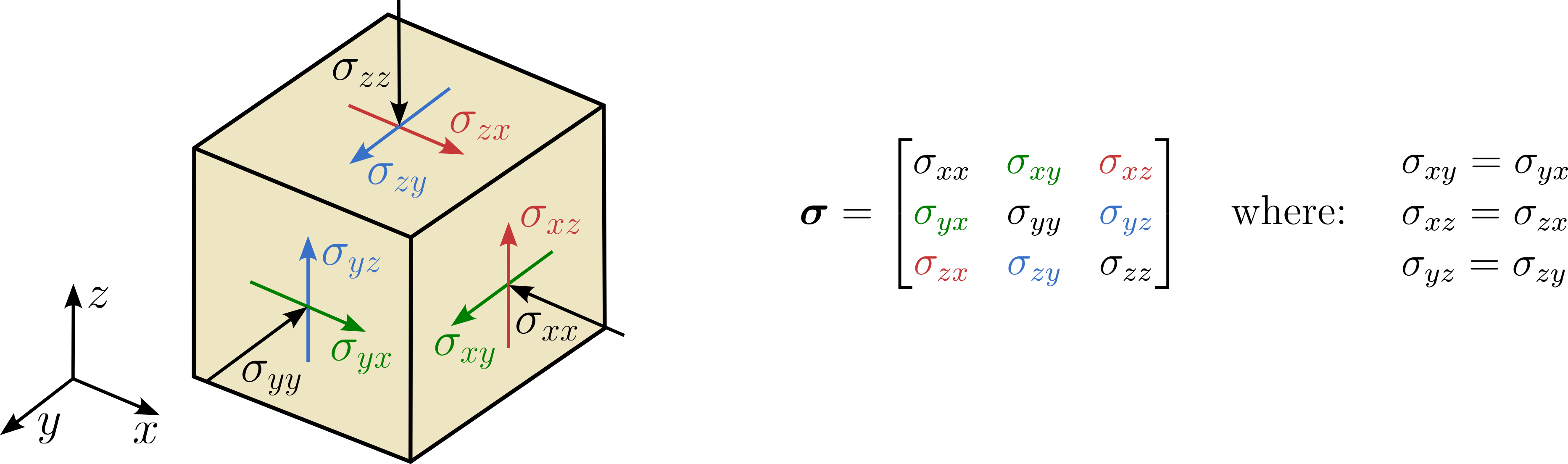
In index notation, the first index of the stress component denotes the plane in which the stress is acting and the second index denotes its direction. Example: the shear stress component \(\sigma_{xy}\) is acting in the \(x\)-plane and pointing in the \(y\)-direction.

A stress tensor can be separated into two portions: volumetric and deviatoric. The deviatoric stress \(\sigma^*\) is a tensor with null trace, and is then defined as:

\[ \sigma_{ij}^* = \sigma_{ij} - \dfrac{1}{3} \sigma_{kk} \delta_{ij} \]

Principal stresses

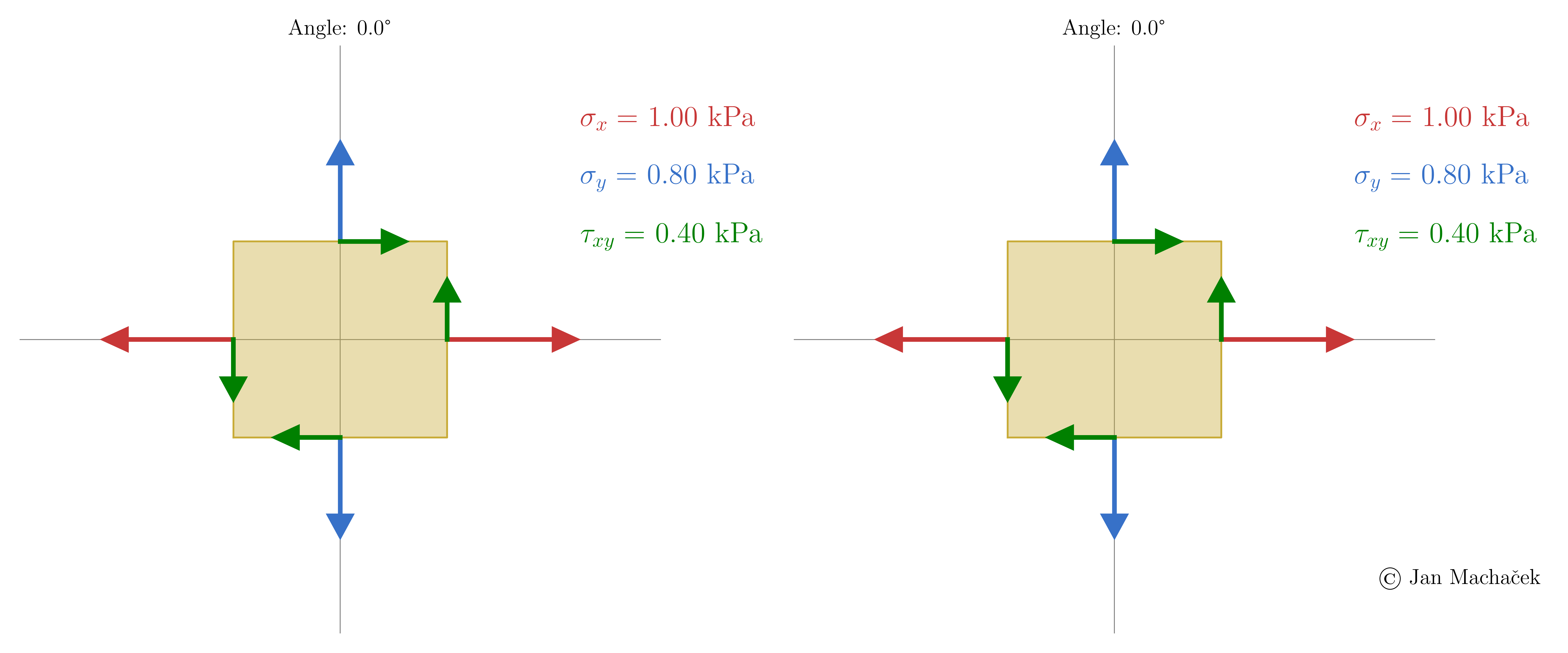
In any stressed body, it is possible to identify three mutually perpendicular planes on which the shear stress vanishes. The normal stresses on these planes, known as principal stresses \(\sigma_{1} > \sigma_{2} > \sigma_{3}\), represent the extremes of normal stress values in the body. The orientations of these planes define the principal directions. Principal stresses emerge when the stress element is oriented such that shear stresses are nullified. This behavior is illustrated for a 2D case in the animation below.

Rotation of stress element to find the principal stresses (click to play)

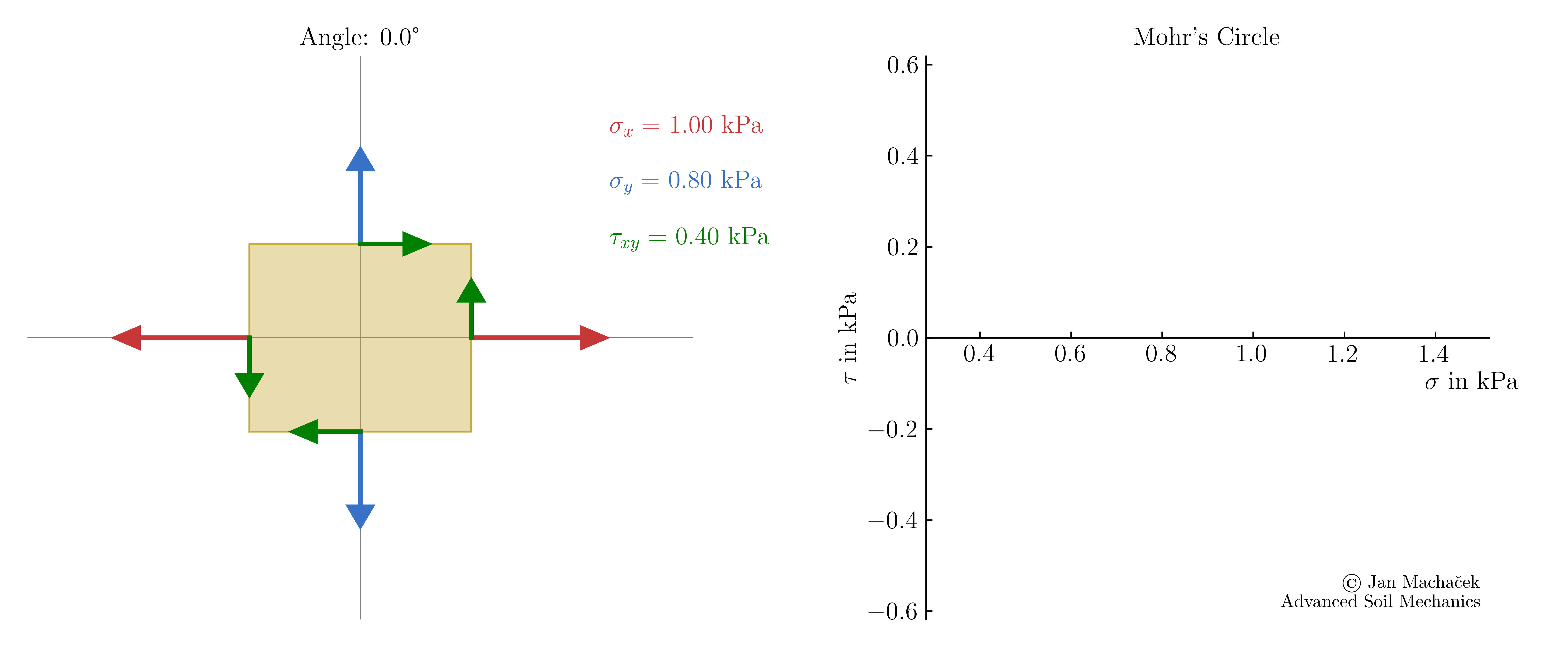
During undergraduate courses, you may have learned a straightforward approach to determining the principal stresses for a given stress state using Mohr's circle, as shown below.

Left: exemplarily 2D stress state, right: construction of Mohr's circle (click to play)

For an algebraic determination of the principal stresses, one can solve the following characteristic equation (often referred to as the eigenvalue problem):

\[ \text{det}\left( T_{ij} - \lambda \delta_{ij} \right) = 0 ~~~\text{where:} ~~~ T_{ij} = -\sigma_{ij} \]

This equation yields a third-order polynomial with three distinct roots (eigenvalues) denoted as \(\lambda^1, \lambda^2, \lambda^3\). These values correspond to the principal stress components \(\sigma_{1}, \sigma_{2}\), and \(\sigma_{3}\).