Stiffness matrix

In the previous section Features of constitutive models for soils we learned that the constitutive description of the non-linear stress-strain behaviour of soils requires in general a non-constant proportionality factor - called stiffness \(E\) - relating stress \(\sigma\) to strain \(\varepsilon\) and wise versa of the form

\[ \dot{\sigma} = E(\sigma,e,sv) \dot{\varepsilon} \]

In above equation, \(E(\sigma,e,sv)\) indicates that the stiffness \(E\) is a function of the soil state defined by the stress \(\sigma\), the void ratio \(e\). The variable \(sv\) indicates that the stiffness can - but not must - depend on other additional state variables \(sv\), depending on the (complexity) of the constitutive model. The rate form is a requirement of the non-linearity of the material behaviour. Alternatively, an incremental relationship can be used

\[ \Delta \sigma = E(\sigma,e,sv) \Delta \varepsilon \]

where \(\Delta \sqcup = \int_{t_0}^{t_1} = \dot{\sqcup} dt = \dot{\sqcup} \Delta t\) was used. Obviously above equations hold for the 1D case only. In general, the stress (rate) and strain (rate) tensors are second order tensors of size 3x3:

\[ \dot{\boldsymbol{\sigma}} = \begin{bmatrix} \dot{\sigma}_{11} & \dot{\sigma}_{12} & \dot{\sigma}_{13} \\ \dot{\sigma}_{21} & \dot{\sigma}_{22} & \dot{\sigma}_{23} \\ \dot{\sigma}_{31} & \dot{\sigma}_{32} & \dot{\sigma}_{33} \end{bmatrix} ~~~ \text{and}~~~ \dot{\boldsymbol{\varepsilon}} = \begin{bmatrix} \dot{\varepsilon}_{11} & \dot{\varepsilon}_{12} & \dot{\varepsilon}_{13} \\ \dot{\varepsilon}_{21} & \dot{\varepsilon}_{22} & \dot{\varepsilon}_{23} \\ \dot{\varepsilon}_{31} & \dot{\varepsilon}_{32} & \dot{\varepsilon}_{33} \end{bmatrix} \]

or in index notation: \(\sigma_{ij}\) and \(\varepsilon_{kl}\), where \(i,j,k\) and \(l\) range from 1 to 3. Therefore the relation ship between these two is a 4th order tensor, here given in index notation:

\[ \dot{\sigma}_{ij} = E_{ijkl} \dot{\varepsilon}_{kl} \]

Since it is not possible to represent all components of a 4th order tensor in a 2D representation, the above equation is usually given either in index or matrix notation, or in flattened form, where the columns (or rows) are stacked on top of each other:

\[ \begin{bmatrix} \dot{\sigma}_{11} \\ \dot{\sigma}_{22} \\ \dot{\sigma}_{33} \\ \dot{\sigma}_{12} \\ \dot{\sigma}_{13} \\ \dot{\sigma}_{23} \\ \dot{\sigma}_{21} \\ \dot{\sigma}_{31} \\ \dot{\sigma}_{32} \\ \end{bmatrix} = \begin{bmatrix} E_{1111} & E_{1122} & E_{1133} & E_{1112} & E_{1113} & E_{1123} & E_{1121} & E_{1131} & E_{1132} \\ E_{2211} & E_{2222} & E_{2233} & E_{2212} & E_{2213} & E_{2223} & E_{2221} & E_{2231} & E_{2232} \\ E_{3311} & E_{3322} & E_{3333} & E_{3312} & E_{3313} & E_{3323} & E_{3321} & E_{3331} & E_{3332} \\ E_{1211} & E_{1222} & E_{1233} & E_{1212} & E_{1213} & E_{1223} & E_{1221} & E_{1231} & E_{1232} \\ E_{1311} & E_{1322} & E_{1333} & E_{1312} & E_{1313} & E_{1323} & E_{1321} & E_{1331} & E_{1332} \\ E_{2311} & E_{2322} & E_{2333} & E_{2312} & E_{2313} & E_{2323} & E_{2321} & E_{2331} & E_{2332} \\ E_{2111} & E_{2122} & E_{2133} & E_{2112} & E_{2113} & E_{2123} & E_{2121} & E_{2131} & E_{2132} \\ E_{3111} & E_{3122} & E_{3133} & E_{3112} & E_{3113} & E_{3123} & E_{3121} & E_{3131} & E_{3132} \\ E_{3211} & E_{3222} & E_{3233} & E_{3212} & E_{3213} & E_{3223} & E_{3221} & E_{3231} & E_{3232} \\ \end{bmatrix} \begin{bmatrix} \dot{\varepsilon}_{11} \\ \dot{\varepsilon}_{22} \\ \dot{\varepsilon}_{33} \\ \dot{\varepsilon}_{12} \\ \dot{\varepsilon}_{13} \\ \dot{\varepsilon}_{23} \\ \dot{\varepsilon}_{21} \\ \dot{\varepsilon}_{31} \\ \dot{\varepsilon}_{32} \\ \end{bmatrix} \]

In above equation, stress and strain are represented by vectors with 9 components and the stiffness matrix as a 9x9 matrix with a total of 81 components. Multiplication is then performed as usual, column by row, here for example for component 11 of the stress rate:

\[ \begin{aligned} \dot{\sigma}_{11} &= E_{11kl}\dot{\varepsilon}_{kl} \\ & = E_{1111}\dot{\varepsilon}_{11} + E_{1122}\dot{\varepsilon}_{22} + E_{1133}\dot{\varepsilon}_{33} \\ & ~~~~+ E_{1112}\dot{\varepsilon}_{12} + E_{1113}\dot{\varepsilon}_{13} + E_{1123}\dot{\varepsilon}_{23}\\ & ~~~~+ E_{1121}\dot{\varepsilon}_{21} + E_{1131}\dot{\varepsilon}_{31} + E_{1132}\dot{\varepsilon}_{32} \end{aligned} \]

Symmetry of stress and strain (Voigt notation)

Usually symmetry of the stress and strain tensors are assumed, i.e

\[ \begin{aligned} \sigma_{12} = \sigma_{21} ~~~,~~~ \sigma_{13} = \sigma_{31} ~~~,~~~ \sigma_{23} = \sigma_{32}\\ \varepsilon_{12} = \varepsilon_{21} ~~~,~~~ \varepsilon_{13} = \varepsilon_{31} ~~~,~~~ \varepsilon_{23} = \varepsilon_{32} \end{aligned} \]

which allows to rewrite the equation for \(\dot{\sigma}_{11}\) as follows:

\[ \dot{\sigma}_{11} = E_{1111}\dot{\varepsilon}_{11} + E_{1122}\dot{\varepsilon}_{22} + E_{1133}\dot{\varepsilon}_{33} + 2E_{1112}\dot{\varepsilon}_{12} + 2E_{1113}\dot{\varepsilon}_{13} + 2E_{1123}\dot{\varepsilon}_{23} \]

Exploiting the symmetry of the stress and strain tensors leads to a condensed representation of the stress-strain relationship usually referred to as Voigt notation:

\[ \begin{bmatrix} \dot{\sigma}_{11} \\ \dot{\sigma}_{22} \\ \dot{\sigma}_{33} \\ \dot{\sigma}_{23} \\ \dot{\sigma}_{13} \\ \dot{\sigma}_{12} \\ \end{bmatrix} = \begin{bmatrix} E_{1111} & E_{1122} & E_{1133} & E_{1123} & E_{1113} & E_{1112} \\ E_{2211} & E_{2222} & E_{2233} & E_{2223} & E_{2213} & E_{2212} \\ E_{3311} & E_{3322} & E_{3333} & E_{3323} & E_{3313} & E_{3312} \\ E_{2311} & E_{2322} & E_{2333} & E_{2323} & E_{2313} & E_{2312} \\ E_{1311} & E_{1322} & E_{1333} & E_{1323} & E_{1313} & E_{1312} \\ E_{1211} & E_{1222} & E_{1233} & E_{1223} & E_{1213} & E_{1212} \\ \end{bmatrix} \begin{bmatrix} \dot{\varepsilon}_{11} \\ \dot{\varepsilon}_{22} \\ \dot{\varepsilon}_{33} \\ 2\dot{\varepsilon}_{23} \\ 2\dot{\varepsilon}_{13} \\ 2\dot{\varepsilon}_{12} \\ \end{bmatrix} \]

Compared to the full notation, in Voigt notation, the stiffness tensor is represented by a 6x6 matrix with 36 components (instead of a 9x9 matrix with 81 components).

Symmetry of \(E_{ijkl}\)

The symmetry of the stress and strain tensors do not imply symmetry of the stiffness tensor \(E_{ijkl}\). In general, \(E_{ijkl}\) is un-symmetric. Only in special cases, for example for isotropic elasticity, \(E_{ijkl}\) is symmetric.

The role of constitutive models is to provide mathematical relationships to calculate the components of the stiffness tensor. Three simple constitutive models are discussed in the following sections.

Isotropic or anisotropic stiffness?

Laboratory tests show that soil behaviour is often anisotropic. This means that the stiffness is not identical in all spatial directions. If a soil sample is loaded with a given strain increment \(\Delta \varepsilon = \Delta \varepsilon_v = \Delta \varepsilon_h\) once in the vertical direction \(v\) and once in the horizontal direction \(h\), this will result in two non-identical stress increments \(\Delta \sigma_v \neq \Delta \sigma_h\). Assumptions relevant to geotechnics regarding (an)isotropy are

Isotropic stiffness: The stiffness is identical in all directions
Transversal anisotropic stiffness: The stiffness is identical in the two horizontal directions but different from the vertical direction. Due of soil formation by sedimentation, this is a particularly relevant case for geotechnical engineering, especially for fine grained soils with rather elongated flat particles such as clays.
Orthotropic stiffness: The stiffness is different for all three directions

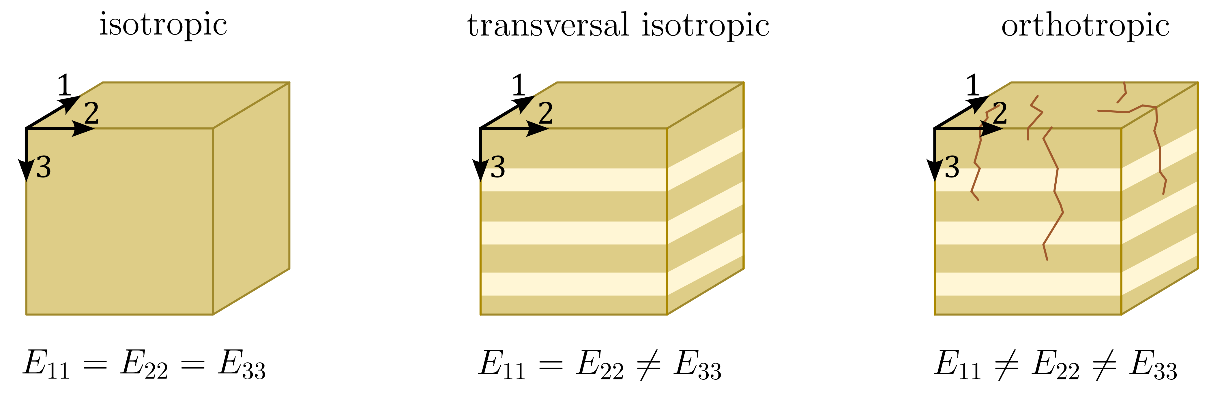
Figure 1. Schematic representation of isotropic, transversal isotropic or orthotropic materials.

Isotropic stiffness

Isotropy means that no direction is distinguished in the material behaviour, i.e. the stiffness is identical in all three directions, from which follows that

All normal components are identical, i.e.

\(E_{1111}=E_{2222}=E_{3333}\)
All normal-normal coupling terms are identical, i.e.

\(E_{1122}=E_{1133}=E_{2211}=E_{2233}=E_{3311}=E_{3322}\)
All shear-shear coupling terms are identical, i.e.

\(E_{1212}=E_{2121}=E_{1313}=E_{3131}=E_{2323}=E_{3232}\)

Thus only three independent components exist: \(E_{1111}, E_{1122}\) and \(E_{1212}\). In Voigt notation the stiffness tensor of an isotropic material reads:

\[ \mathbf{E} = \begin{bmatrix} E_{1111} & E_{1122} & E_{1122} & 0 & 0 & 0 \\ E_{1122} & E_{1111} & E_{1122} & 0 & 0 & 0 \\ E_{1122} & E_{1122} & E_{1111} & 0 & 0 & 0 \\ 0 & 0 & 0 & E_{1212} & 0 & 0 \\ 0 & 0 & 0 & 0 & E_{1212} & 0 \\ 0 & 0 & 0 & 0 & 0 & E_{1212} \\ \end{bmatrix} \]

Transversal isotropic stiffness

Transverse isotropy (or transversely isotropic materials) have a unique axis of symmetry. This means that properties in the plane perpendicular to this axis are isotropic, but properties along the axis may be different. This is illustrated in Figure 1, where the axis of symmetry is axis 3. For a material with transverse isotropy, there are five independent stiffness constants. These are typically denoted as \(E_{1111}\), \(E_{1122}\), \(E_{1133}\), \(E_{1212}\) and \(E_{2323}\) (or \(E_{1313}\)).

In Voigt notation, the stiffness matrix for a transversely isotropic material can be written as:

\[ \mathbf{E} = \begin{bmatrix} E_{1111} & E_{1122} & E_{1133} & 0 & 0 & 0 \\ E_{1122} & E_{1111} & E_{1133} & 0 & 0 & 0 \\ E_{1133} & E_{1133} & E_{3333} & 0 & 0 & 0 \\ 0 & 0 & 0 & E_{1212} & 0 & 0 \\ 0 & 0 & 0 & 0 & E_{1212} & 0 \\ 0 & 0 & 0 & 0 & 0 & E_{1313} \\ \end{bmatrix} \]

In this matrix:

\(E_{1111} = E_{2222}\) represent the stiffness in the plane of isotropy.
\(E_{1133} = E_{2233}\) represent the stiffness due to a strain along the axis of symmetry from stress in the isotropic plane.
\(E_{3333}\) represents the stiffness along the axis of symmetry.
\(E_{1212}\) is the in-plane shear modulus.
\(E_{1313} = E_{2323}\) represent the out-of-plane shear modulus.

In transverse isotropy, \(E_{1212}\) is equivalent to \(E_{2323}\) due to the isotropic response within the transverse plane, and they are typically denoted by a single shear modulus, often referred to as \(G\) in literature. The above matrix reflects the symmetry and coupling in a transversely isotropic material.