Invariants

In the context of granular media, such as soils, stress represents an averaged measure of the contact forces between grains over a representative volume. As such, the intricate details of force chains are captured within a continuous and differentiable stress field, which provides both the magnitude and orientation of the averaged contact forces.

Stress invariants

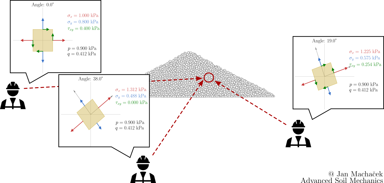
Stress tensors, being multi-dimensional entities, can be difficult to work with. Stress invariants simplify the representation of stress states into scalar quantities, making mathematical and graphical analyses more tractable. Stress invariants, by definition, remain unchanged regardless of the orientation of the coordinate system. This property ensures that the derived quantities and predictions based on them are consistent regardless of the observer's orientation, as illustrated below.

The invariants of the stress tensor, commonly presented in textbooks on continuum mechanics, are defined as:

\[ \begin{aligned} I_1 &= T_1 + T_2 + T_3 \\ I_2 &= T_1T_2 + T_2T_3 + T_3T_1 \\ I_3 &= T_1T_2T_3 \end{aligned} \]

For the deviatoric invariants of the stress tensor \(T^*\), the definitions are:

\[ \begin{aligned} J_1 &= 0 \\ J_2 &= \frac{1}{2} \left( T^*_{ij} T^*_{ji} \right) \\ J_3 &= \text{det}(T^*) \end{aligned} \]

However, in geotechnical engineering, the Roscoe (Cambridge) invariants, particularly \(q\) (deviatoric stress) and \(p\) (mean stress), are favoured due to their direct relevance to soil behaviour. The mean stress \(p\) reflects the overall confining pressure in soils, while \(q\) relates to shearing behaviour. These invariants align well with the Mohr-Coulomb failure criterion, a foundational concept in soil mechanics. The introduction of critical state soil mechanics, which utilizes \(p\) and \(q\), further underscores their importance. Their simplicity offers intuitive insights into practical geotechnical problems. Historically, geotechnical theories and education have been built around these invariants, solidifying their use in the field.

Roscoe Invariants

By this point in your studies, you likely have experience interpreting the results of laboratory tests in terms of principal stresses, e.g. looking at the results from a triaxial compression test in terms of the development of deviatoric stress \(q\) over axial strain \(\varepsilon_{ax}\) as shown below.

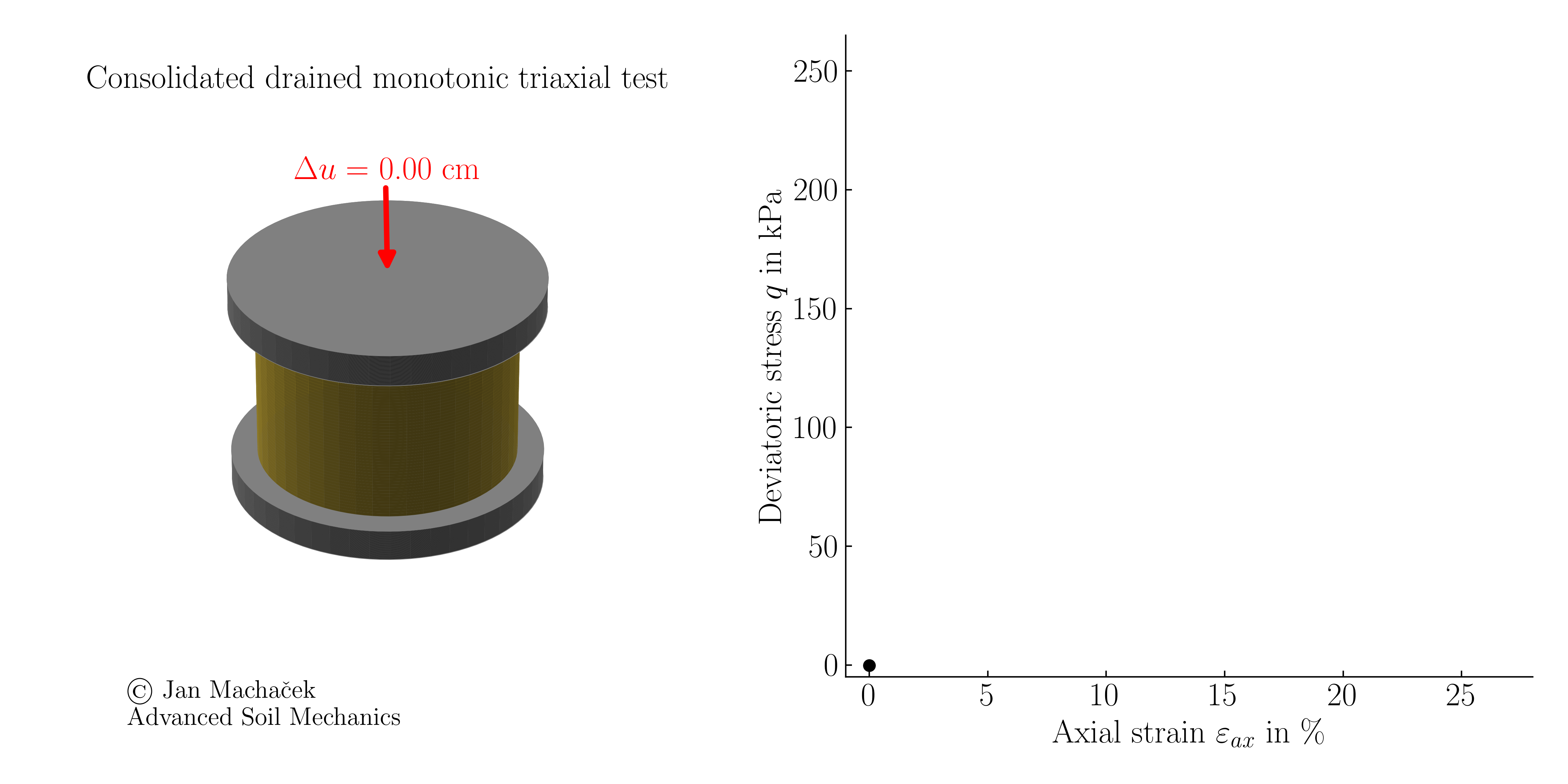Consolidated drained monotonic triaxial test (click to play)

Understanding the stress state in a material is foundational for interpreting laboratory tests and modeling behaviour. This fundamental concept becomes even clearer when we introduce the Roscoe invariants. These scalar representations, denoted as \(p\) and \(q\), bridge our knowledge of stress states with tangible metrics that have deep-rooted applications in geotechnics. These invariants are related to the stress tensor \(\boldsymbol{T}=-\sigma_{ij}\). Their definitions for general stress states are given by:

\[ \begin{aligned} p &= \dfrac{1}{3} \text{tr}(\boldsymbol{T}) = \dfrac{1}{3} \delta_{ij} \sigma_{ij} = \dfrac{1}{3} \sigma_{ii} \quad \text{(Mean Stress)} \\ q &= \sqrt{ \dfrac{3}{2} \boldsymbol{T}^* : \boldsymbol{T}^* } \quad \text{(Deviatoric Stress Magnitude)} \end{aligned} \]

The first Roscoe invariant, \(p\), is commonly referred to as the mean (effective) stress or (mean) pressure. It encapsulates the volumetric component of the stress tensor. A frequent application is its role in delineating the dependency of soil stiffness on the mean effective stress, a phenomenon termed barotropy. In a hydrostatic state where the stress in every direction is equal, \(p\) would represent that hydrostatic stress.

Conversely, the second Roscoe invariant, \(q\), zeroes in on the purely deviatoric component of the stress tensor. It's an essential metric for capturing the shear strength of soils, pivotal in assessing soil stability and behaviour under external loads.

Alternatively the Roscoe invariants can also be computed from the principal stresses (\(T_1=-\sigma_{1}, T_2=-\sigma_{2}, T_3=-\sigma_{3}\)) as follows:

\[ \begin{aligned} p &= - \dfrac{1}{3} \left( T_1 + T_2 + T_3 \right) \\ q &= \sqrt{ 3 J_2 } \quad \text{with: } J_2 = \frac{1}{3} \left( T_1^2 + T_2^2 + T_3^2 - \left( T_1T_2 + T_2T_3 + T_3T_1 \right) \right) \end{aligned} \]

The integrative application of both these invariants aids not only in visualising and interpreting numerous laboratory tests on soils but also underpins the foundation of constitutive models in geotechnics. These invariants will prove to be indispensable tools throughout this course and remain essential for both professionals and researchers in the field.

Limitations of Roscoe invariants

For completeness, it's worth mentioning that Roscoe invariants have a limitation: they don't accurately represent the length and inclination when plotting stress or strain vectors¹². Nonetheless, these invariants can be scaled to isometric (isomorphic) quantities \(P = \sqrt{3}p\) and \(Q = \sqrt{\frac{3}{2}}q\). This detail, however, won't significantly impact the topics covered in this lecture.

Lode angle

The Roscoe invariants, represented by \(p\) and \(q\), can be visualized in the principal stress space, as demonstrated in the provided animation (click to initiate). This animation elucidates a methodical procedure to visualize these invariants, and in the process, introduces the concept of the Lode angle.

Representation of Roscoe invariants \(p\) and \(q\) in the principal stress state and introduction of the Lode angle \(\theta\) (click to play). The individuall steps are described in detail below.

The outlined steps are:

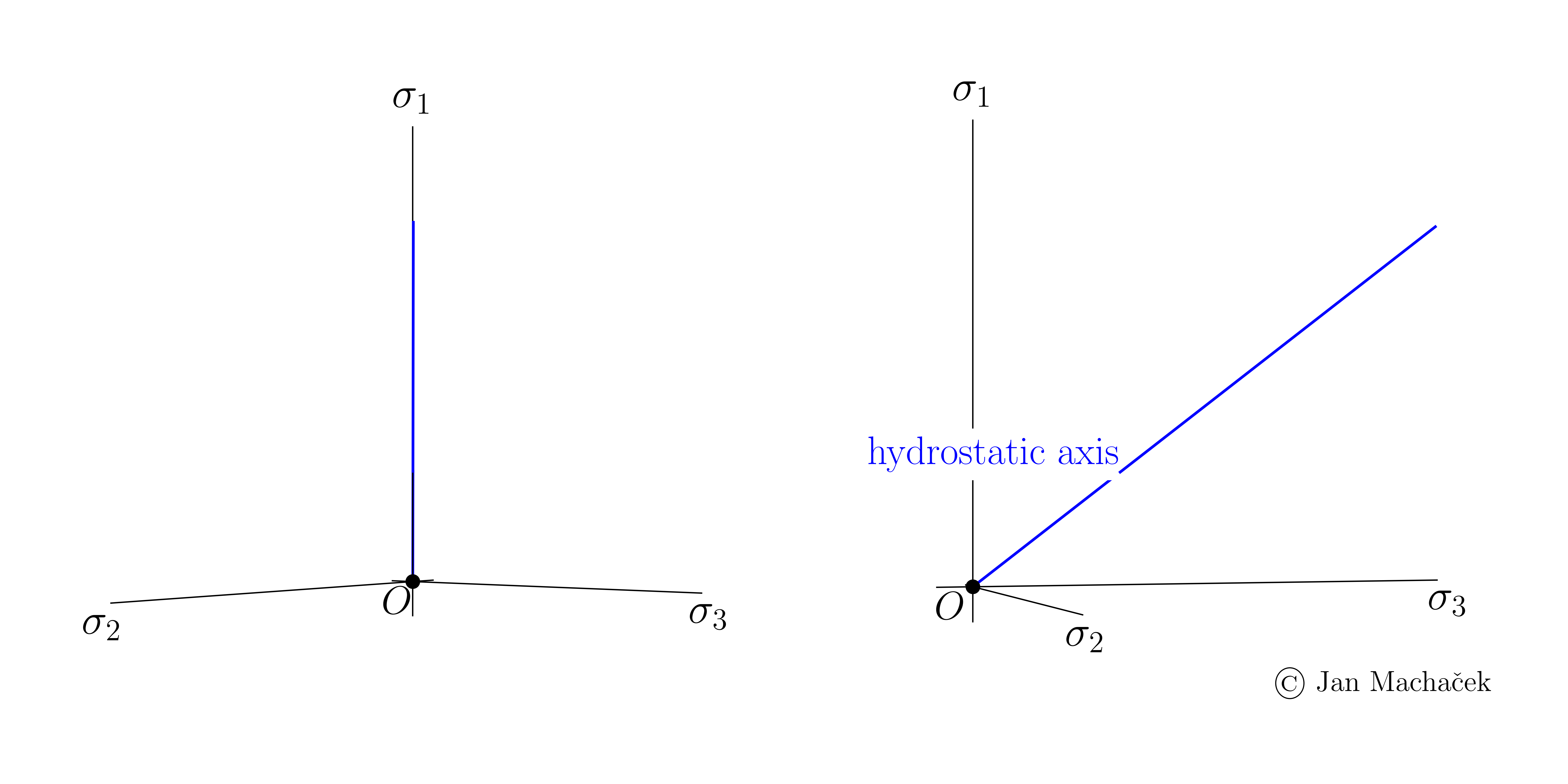
1. Hydrostatic Axis Introduction: Begin with the hydrostatic axis (also known as the space diagonal, blue line in above figure). Along this axis, the equation \(\sigma_1 = \sigma_2 = \sigma_3\) is valid. The Roscoe invariant \(p=(\sigma_1+\sigma_2+\sigma_3)/3\) (mean stress) will be projected along this axis at a subsequent step.

   Note

   Note that the distance between the origin and the point on the hydrostatic axis is \(\overline{OA}=\sqrt{3}p\). This is a consequence of the geometric representation in the principal stress space. The length (or magnitude) of the position vector to the hydrostatic point is formed as the diagonal of a cube in the principal stress \(\overline{OA}=\sqrt{\sigma_1^2+\sigma_2^2+\sigma_3^2}\). Considering \(\sigma_1 = \sigma_2 = \sigma_3 = p\) yields \(\overline{OA}=\sqrt{3}p\).

2. Deviatoric Plane Construction: Erect a plane perpendicular to the hydrostatic axis. This is termed the deviatoric plane. Points on this plane represent different deviatoric stresses but maintain the same mean stress. The magnitude of the deviatoric stress at a point is dependent on its distance from the hydrostatic axis.

3. Stress Point Addition: Incorporate a specific stress point into the plot. Initially, this stress state is purely isotropic, implying an absence of deviatoric stress. Consequently, point A is situated on the hydrostatic axis.

4. Stress State Modification: As we progress, the stress state undergoes changes. While the mean stress remains unchanged, the deviatoric stress sees an augmentation. This transformed stress state is represented by the red point B. Observably, with a rise in deviatoric stress, the distance AB expands. Precisely, the length of segment AB equals \(\sqrt{\frac{2}{3}}q\).

5. Lode Angle Measurement: Finally, measure the angle between the hypothetical line joining A and the intersection of the deviatoric plane with the \(\sigma_1\) plane and the line that traverses through AB. This measured angle is termed the Lode angle, the implications of which will be delved into subsequently.

The Lode angle, denoted as \(\theta\), is named after André Lode and serves as a parameter to describe the orientation of the stress state within the deviatoric stress space. It encapsulates the interrelations and relative magnitudes of the principal stresses, \(\sigma_1\), \(\sigma_2\), and \(\sigma_3\) — representing the maximum, intermediate, and minimum normal stresses, respectively, on a material element. Without loss of generality Lodes angle can be calculated from

\[ \cos(3\theta) = -\dfrac{3 \sqrt{3}J_3}{2 J_2^{3/2}} ~~~\text{with}~~~ \theta \in [0,\pi/3] \]

For \(\sigma_1 > \sigma_2 > \sigma_3\) above equation can be rewritten as follows:

\[ \theta = \arctan \left( \sqrt{3} \dfrac{b}{2-b} \right) ~~~\text{with}~~~ b = \dfrac{\sigma_2-\sigma_3}{\sigma_1-\sigma_3} \]

Significance for geotechnical engineering In order to fully describe 3D stress states, either the full stress tensor or the Roscoe invariants \(p\) and \(q\) together with the Lode angle \(\theta\) are required. Note that from \(p\) and \(q\) alone, the full stress tensor can not be recovered, as multiple combinations of stress components \(\sigma_{ij}\) exist that lead to the same \(p\) and \(q\) (see e.g. the figure at the top of this page). In geotechnical engineering, the Lode's angle is frequently utilized to describe the constitutive behaviour of soil. Many failure criteria are formulated in terms of the principal stresses \(p\) and \(q\), with the Lode's angle serving to incorporate information regarding the orientation of the stress state. One such failure criterion that you might already be familiar with is the Mohr-Coulomb failure criterion. The representation of this criterion in the principal stress space is provided below.

More animations

Excellent interactive graphical representations of different widely used failure criteria such as Mohr-Coulomb, Drucker-Prager, Tresca, von Mises and Matsuoka-Nakai have been created by Gertraud Medicus and are provided free of charge here (sign-up required). Having a look at these is highly recommended.

Strain invariants

The strain invariants corresponding to the Roscoe stress invariants are \(\varepsilon^{vol}\) and \(\varepsilon^q\) and are defined as follows:

\[ \begin{aligned} \varepsilon^{vol} &= \delta_{ij}\varepsilon_{ij} = \varepsilon_{11} + \varepsilon_{22} + \varepsilon_{33} = \varepsilon_x + \varepsilon_y + \varepsilon_z \\ \varepsilon^q &= \sqrt{ 3 \varepsilon_{ij}^\ast \varepsilon_{ij}^\ast } \end{aligned} \]

where \(\delta_{ij}\) is the Kronecker-Delta and \(\varepsilon_{ij}^\ast\) is the deviatoric portion of the strain tensor. While the definition of \(\varepsilon^q\) is similar to the Roscoe stress invariant \(q\), the definition of the \(\varepsilon^{vol}\) differs from \(p\). This difference arises from the physical significance of stress and strain. Stress invariants, such as the mean stress, offer insights into force equilibrium, and material response, while strain invariants provide a measure of the deformation experienced by a material. The absence of the \(1/3\) factor in the volumetric strain invariant \(\varepsilon^{vol}\) comes from the fact that the volumetric strain directly quantifies the relative change in volume, unlike the mean stress where we're averaging the normal stresses.

---

1. A. Niemunis and C. Karcher, Theoretische Bodenmechanik mit Mathematica. 2022. ↩

2. F. Prada, Presentation: Introduction to Tensor Calculus, Advanced Constitutive Models for Geomaterials (WP44), Ruhr-Universität Bochum, 14th April 2023 ↩