Triaxial test (on sand)

Be aware that...

This chapter does not aim to thoroughly introduce the students to the topic of triaxial tests on soils. Its intention is rather to refresh what is already known and introduce some key features of triaxial tests, in particular drained monotonic triaxial tests on sand. For a complete introduction to triaxial testing on soils, study of ² and ³ is recommended. Important topics such as the influence of sample size/geometry and boundary conditions, the sample preparation method (see ¹ amongst others), the influence of sample saturation as well as questions related to the required extent of the experimental campaign (number of tests) are not discussed.

After a brief introduction and some notes on the evaluation of triaxial tests, we will start by looking at the basics of three different triaxial tests:

• Consolidated drained monotonic triaxial tests on sand
• Consolidated undrained monotonic triaxial tests on sand
• Consolidated undrained monotonic triaxial extension tests on sand

To this point, we will have limited discussion to the influence of the density and the loading direction (compression vs. extension) on the behaviour of sands. The influence of the mean effective stress \(p^\prime\), known as barotropy, was not yet considered and is covered in

• Influence of mean effective pressure

which exemplarily demonstrates how the initial (effective) stress affects the experiments presented earlier.

Introduction

Triaxial (compression) tests are widely used laboratory tests to investigate the shear strength soils. A typical triaxial testing device is depicted below.

Slider 1: Schematic representation of the setup of a triaxial testing device

The soil specimen is cylindrical and is enveloped by a rubber membrane. This specimen is bounded at the top and bottom by end plates (top-cap and pedestal), both incorporating porous discs for drainage. The specimen resides in a cell typically made of clear Perspex or acrylic, allowing for visual observations. A liquid pressure, denoted as \(\sigma_3^\prime\), confines the specimen. The eventual yielding or failure of the soil specimen is triggered by a gradually increasing axial force \(F\), leading to an increase in axial stress \(\sigma_1^\prime\). The sample is usually saturated with deaired water, so that its volume change is measured by the amount of water squeezed out. It's worth noting that, contrary to what the name "triaxial" might suggest, the stress state within the soil specimen during this test is axisymmetric. This means that stresses are symmetric about the central axis of the specimen and not truly triaxial in nature.

As discussed in Simplified stress conditions, triaxial loading conditions further imply that:

• The confining pressure is applied uniformly in all radial directions. As a result, there are no differential stresses acting tangentially on the specimen's surface, eliminating the possibility of shear strain in the radial direction.
• The axial load applied to the specimen is vertical and acts along the central axis of the cylindrical specimen. Because of this, there's no lateral component of the axial load that might introduce shear.
• The cylindrical shape of the specimen ensures that the state of stress at any given point within the specimen remains consistent (given that the sample is homogenous). This means that, theoretically, no rotational or tangential stresses develop within the specimen due to its shape.
• The top and bottom plates of the triaxial apparatus ensure that the applied load remains axial and prevents any lateral movement or rotation of the sample. Thus no shear strains are introduced due to the boundary conditions.
• The sample is isotropically confined, thus \(\sigma_2^\prime = \sigma_3^\prime\) holds.

leading to the following simplified stress and strain tensor under triaxial conditions

\[ \boldsymbol{\sigma}^\prime = \begin{bmatrix} \sigma_3^\prime & 0 & 0 \\ 0 & \sigma_3^\prime & 0 \\ 0 & 0 & \sigma_{1}^\prime \\ \end{bmatrix} ~~~\text{and}~~~ \boldsymbol{\varepsilon} \begin{bmatrix} \varepsilon_3 & 0 & 0 \\ 0 & \varepsilon_3 & 0 \\ 0 & 0 & \varepsilon_{1} \\ \end{bmatrix} \]

In above equations \(\sigma_r^\prime\) and \(\sigma_{ax}^\prime\) are replaced by the minimum and maximum principal stress \(\sigma_3^\prime\) and \(\sigma_1^\prime\), respectively. The axial deformation \(\varepsilon_1\) is measured by means of the displacement of the load piston or top-cap. The volumetric deformation \(\varepsilon_v\) is determined by measuring the water out- or inflow into the specimen. The radial deformation \(\varepsilon_3\) can either be measured ''locally'' using circumferential measuring bandages or indirectly from the axial and volumetric strain, i.e. \(\varepsilon_3 = (\varepsilon_v - \varepsilon_1)/2\).

Evaluation

Model presentation for calculating stresses and strains during a triaxial test is given in the figure below. Therein, \(h\) and \(V\) are the current height and volume of the specimen, respectively. \(h_0\) and \(V_0\) are the respective initial values before the start of shearing. Above relations imply the assumption that the sample deforms uniformly and that its diameter remains relatively constant throughout its height.

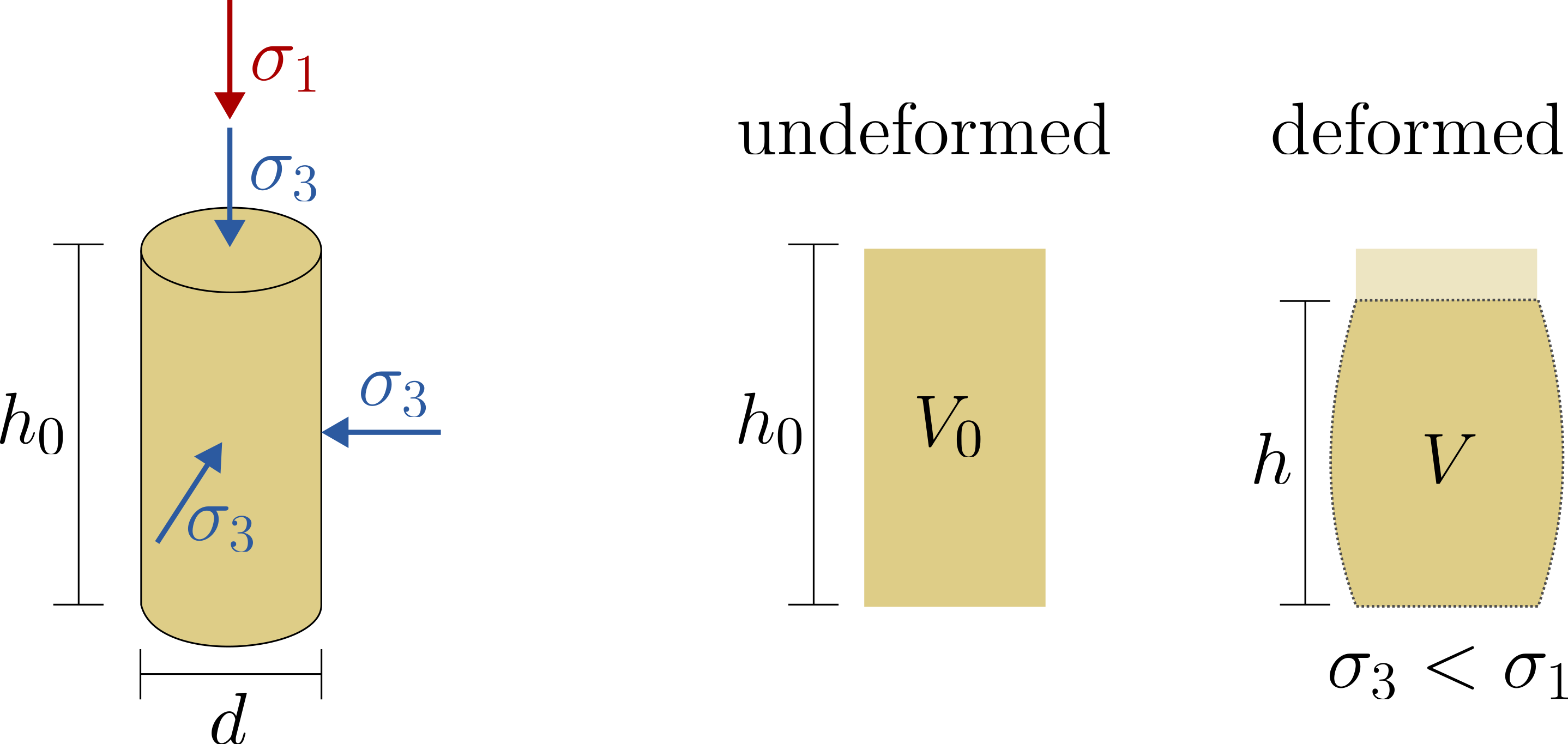
Model presentation for calculating stresses and strains during a triaxial test.

Following above representations, the strains can be calculated as follows:

• Axial strain: \(\varepsilon_1 = \dfrac{h-h_0}{h_0}\)

• Volumetric strain: \(\varepsilon_v = \dfrac{V-V_0}{V_0}\)

• Radial strain: \(\varepsilon_3 = \left( \varepsilon_v-\varepsilon_1 \right) / 2\)

• Deviatoric strain: \(\varepsilon^q = 2 \left( \varepsilon_1- \varepsilon_3 \right)/3\)

• Shear strain: \(\gamma = \varepsilon_1 - \varepsilon_3\)

Evaluation of triaxial tests is typically conducted using one of the following frameworks:

• The traditional representation using mean effective stress \(\sigma_m=(\sigma_1^\prime+\sigma_3^\prime)/2\) and shear stress \(\tau = (\sigma_1^\prime-\sigma_3^\prime)/2\).
• The Roscoe invariants, wherein the mean effective stress (or pressure) is given by \(p^\prime=(\sigma_1^\prime+2\sigma_3^\prime)/3\) and the deviatoric stress is represented as \(q=\sigma_1^\prime-\sigma_3^\prime = 2 \tau\).

\(\tau-\sigma_m\) or \(p^\prime-q\)?

Both these methods provide consistent insight into soil behaviour. While the evaluation using shear stress \(\tau\) is extensively utilized in both educational settings and the industry due to its simplicity and directness, the Roscoe invariant representation offers a more refined approach. Using \(p^\prime\) and \(q\) allows behaviour to be contextualized in terms of invariant measures, which becomes particularly beneficial when delving into the constitutive modelling of soil behaviour. Given that this course intends to introduce to the concept of Critical State Soil Mechanics and will later delve into constitutive modelling, our focus will primarily be on the representation using Roscoe invariants.

---

1. T. Wichtmann and T. Triantafyllidis, ‘An experimental database for the development, calibration and verification of constitutive models for sand with focus to cyclic loading: part I—tests with monotonic loading and stress cycles’, Acta Geotech., vol. 11, no. 4, pp. 739–761, Aug. 2016, doi: 10.1007/s11440-015-0402-z. ↩

2. M. Budhu, Soil mechanics and foundations, 3rd ed. Hoboken, NJ: Wiley, 2011. ↩

3. D. Kolymbas, Geotechnik: Bodenmechanik, Grundbau und Tunnelbau. Berlin, Heidelberg: Springer Berlin Heidelberg, 2011. ↩