Earthquakes and assessment of liquefaction risk

Introduction

Prior to delving into the causative factors of earthquakes and their consequential impacts on civil engineering structures, it is imperative to contextualize the global repercussions of these seismic events on societal and economic fronts. The chart entitled Natural disasters by type offers a comprehensive overview of the predominant natural hazards on an annual basis from 1970 to 2023. An initial examination may suggest that earthquakes occupy a relatively minor position in comparison to extreme weather events and floods. However, this perspective shifts markedly upon considering the data pertaining to economic damages attributed to various types of natural disasters, as depicted in the secondary tabulation Economic damage... of below figure.

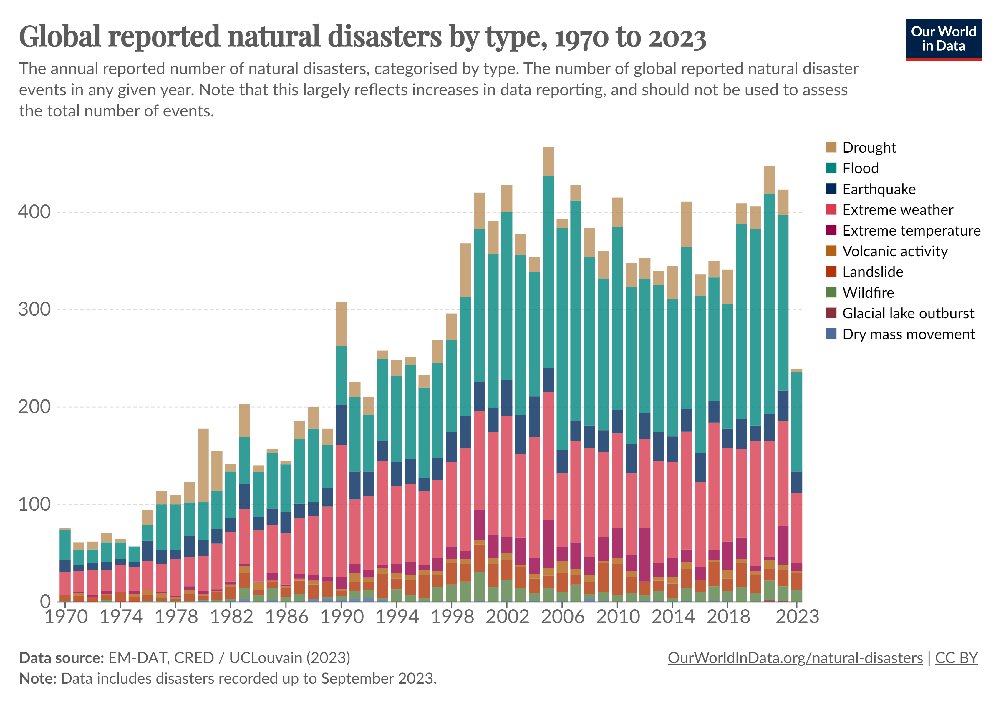
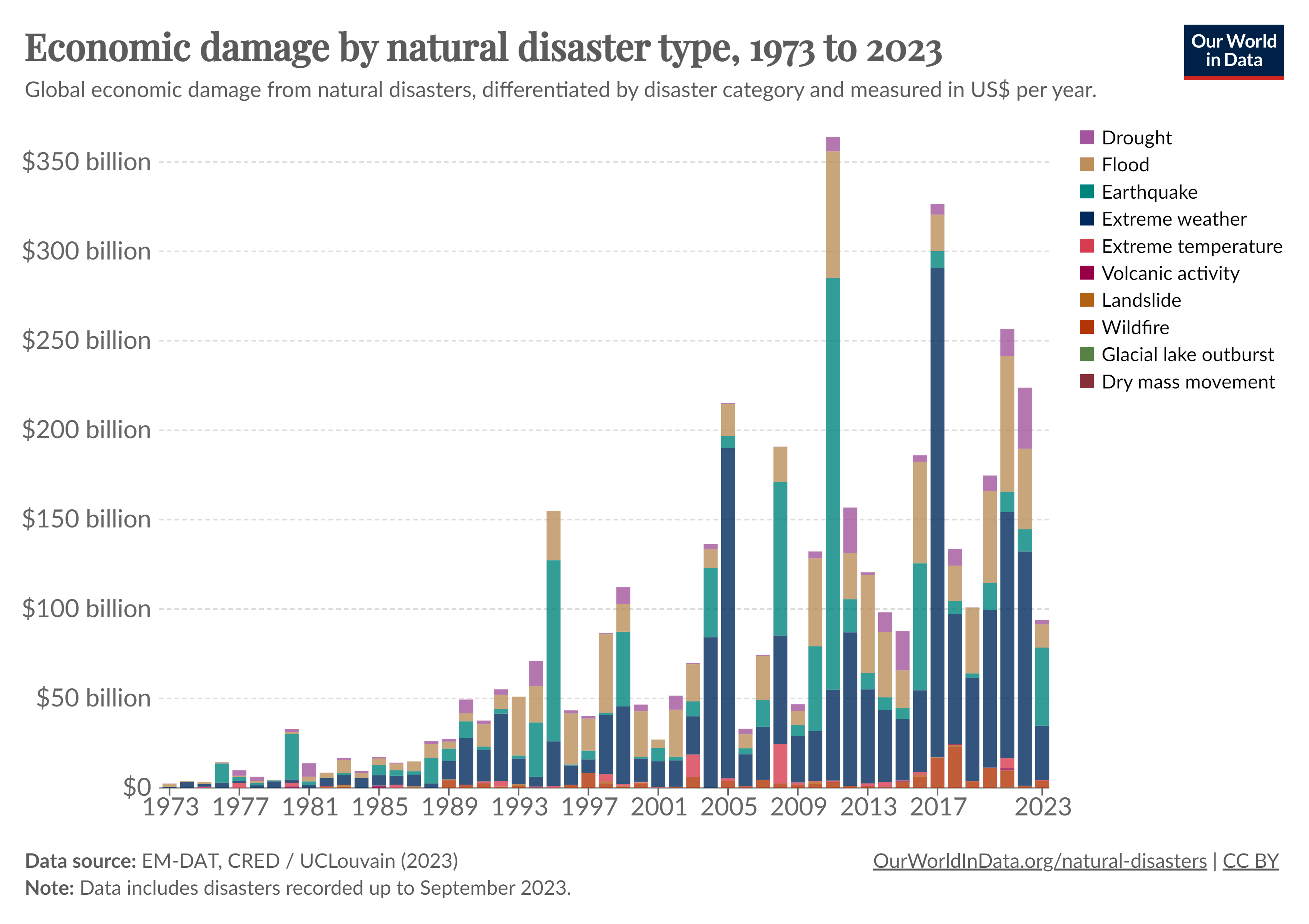
Natural desasters by type, 1970 - 2023Economic damage by natural disaster type, 1973 - 2023

A nuanced analysis reveals that, despite their lower frequency, the economic impact of earthquakes are disproportionately substantial. In certain years, such as 1995, 2008, and 2011, the financial toll inflicted by earthquakes accounted for up to 60 % of the total damages incurred by natural hazards. This underscores the need for a more intricate understanding of seismic phenomena and highlights the critical importance of incorporating seismic considerations in both urban planning and civil engineering practices.

Cause of Earthquakes

Earthquakes represent a fundamental aspect of terrestrial dynamics, primarily emanating from the interactions of tectonic plates within the Earth's lithosphere. These seismic events result from the kinematic interplay of continental and oceanic plates, which undergo relative displacements characterized by divergent, convergent, or tangential movements.

Divergent displacement, where plates move away from each other, often leads to zones of heightened volcanic activity. This process can result in either subsidence of the land or the formation of new mountain ranges, frequently situated below the ocean's water tables. In contrast, convergent displacement involves the subduction of one plate beneath another. This subduction process not only facilitates the melting of the subducting plate but also prompts faulting and uplift in the overriding plate, contributing to the growth of mountain chains.

Additionally, tangential or transform plate movements, characterized by lateral shearing, play a critical role in seismic activity. The movement of these plates is not a continuous process; rather, it is often impeded by the mechanical interlocking of plate boundaries. This leads to a gradual accumulation of shear stress along the fault lines. When the accumulated shear stress surpasses the fault's capacity to withstand it, a sudden displacement occurs, releasing the stored energy as seismic waves - the fundamental cause of an earthquake.

The frequency and magnitude of earthquakes predominantly escalate along tectonic plate boundaries. Notable examples include the Pacific Ring of Fire, where the Pacific Plate encounters various major plates, leading to significant seismic activity along the western coasts of the Americas and in regions like Japan. Similarly, the complex interactions among the African, Arabian, and Indo-Australian plates with the Eurasian plate underscore the global distribution of seismic risks, as depicted in global earthquake risk maps, such as the one shown below.

Earthquake risk in different regions of the world, white/green: low risk, red/brown: very high risk.

The illustrative representation, predominantly shaded green, might convey an impression of a minimal seismic risk in Europe, and by extension, Germany. However, this depiction should not detract from the importance of incorporating seismic considerations into structural design, as mandated by DIN 4149 and its corresponding Eurocode. These standards delineate zones of heightened seismic activity where earthquake-resistant design is imperative.

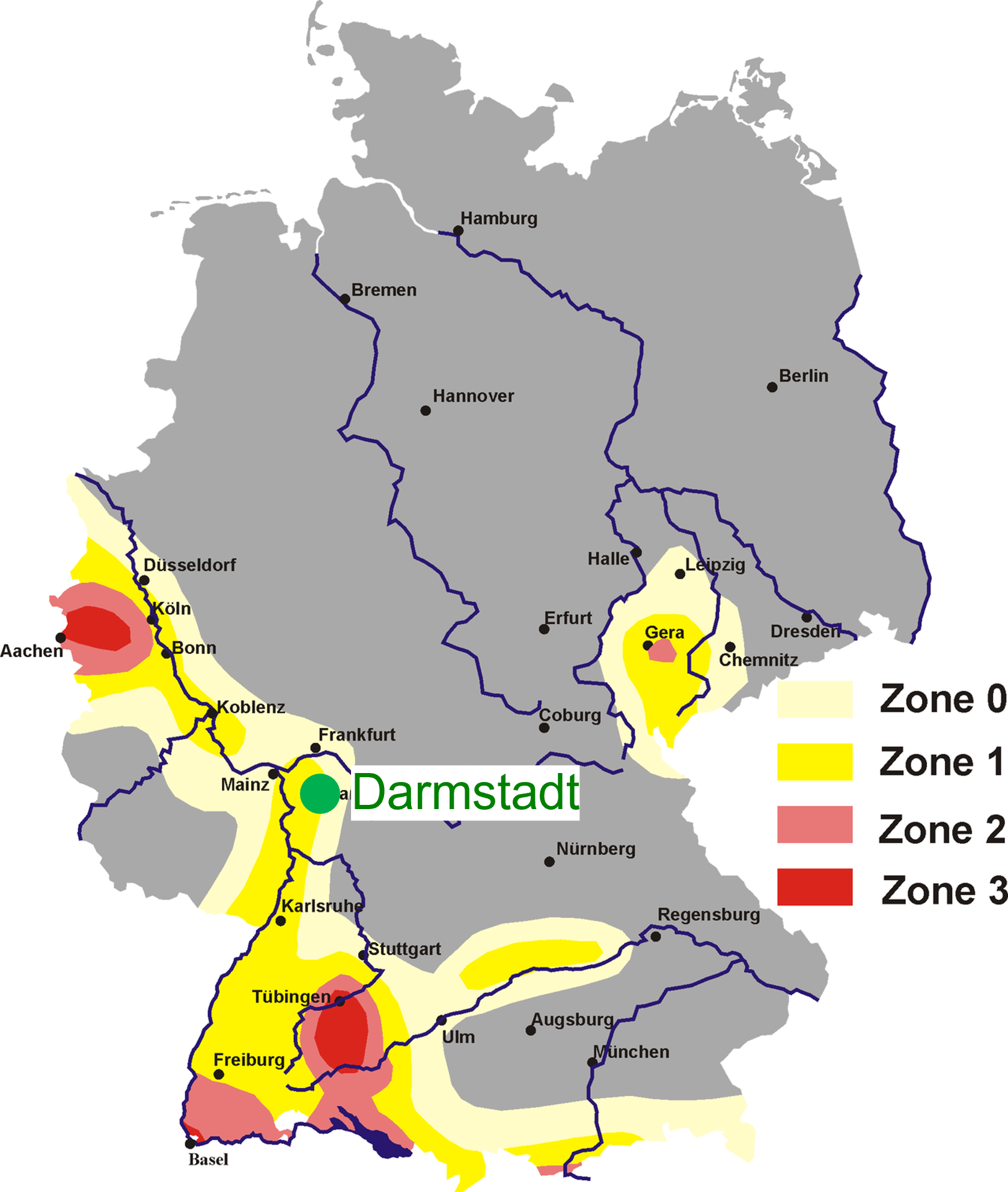
Zones of earthquake risk in Germany according to DIN 4149, modified from ¹

Significant seismic risk is identified in specific regions of Germany, including the area extending between Cologne and the borders with the Netherlands and Belgium, along the Upper Rhine Rift from Frankfurt to Basel, in the vicinity encompassing Stuttgart (more precisely Tübingen) to Lake Constance, and around Gera. The geotectonic underpinnings of these risk zones are rooted in the ongoing collision between the African and Eurasian continental plates. This collisional dynamic not only results in the compression of the Eurasian plate in the direction of the collision but also induces an extension perpendicular to the collision axis. The Rhine River valley, in particular, exemplifies this tectonic activity.

Understanding the seismic effects and accurately assessing the associated risks, such as soil liquefaction, is crucial not only for global engineering practices but also for infrastructure development within Germany and Europe at large. This knowledge is vital for the design and implementation of structures capable of withstanding the seismic forces that these regions may experience, underscoring the need for a comprehensive grasp of regional tectonics and its implications in civil engineering.

Soil liquefaction

Soil liquefaction stands as a critical phenomenon for geotechnical engineers, particularly in the context of earthquake-induced challenges. As introduced in the preceding section, the release of stored energy in the form of seismic waves during tangential tectonic movements is a primary causative factor in earthquakes. These seismic events generate various types of waves, including surface waves, compressional (P-) waves, and shear (S-) waves. For the study of soil liquefaction, the focus predominantly lies on the role of shear waves:

Surface waves, while significant in other aspects of seismic activity, have a secondary impact on the process of soil liquefaction. Their influence is primarily on the ground surface and diminishes with depth, which is less relevant for understanding subsurface soil behavior during seismic events.
Compressional waves, or P-waves, induce simultaneous increases in pore water pressure and total stresses. However, their contribution to changes in effective stress is relatively negligible, thereby rendering them less critical in the context of liquefaction. The primary mechanism of P-waves involves compression and expansion, which does not directly lead to the rearrangement of soil particles necessary for liquefaction.
Shear waves, or S-waves, on the other hand, are instrumental in the phenomenon of soil liquefaction. During shear waves, the soil particles move perpendicular to the direction of wave propagation inducing cyclic shearing strains within the soil. An illustrative animation of shear waves is given in below animation. While the wave propagates from left to right, the particles (illustrated by cells) move up and down.

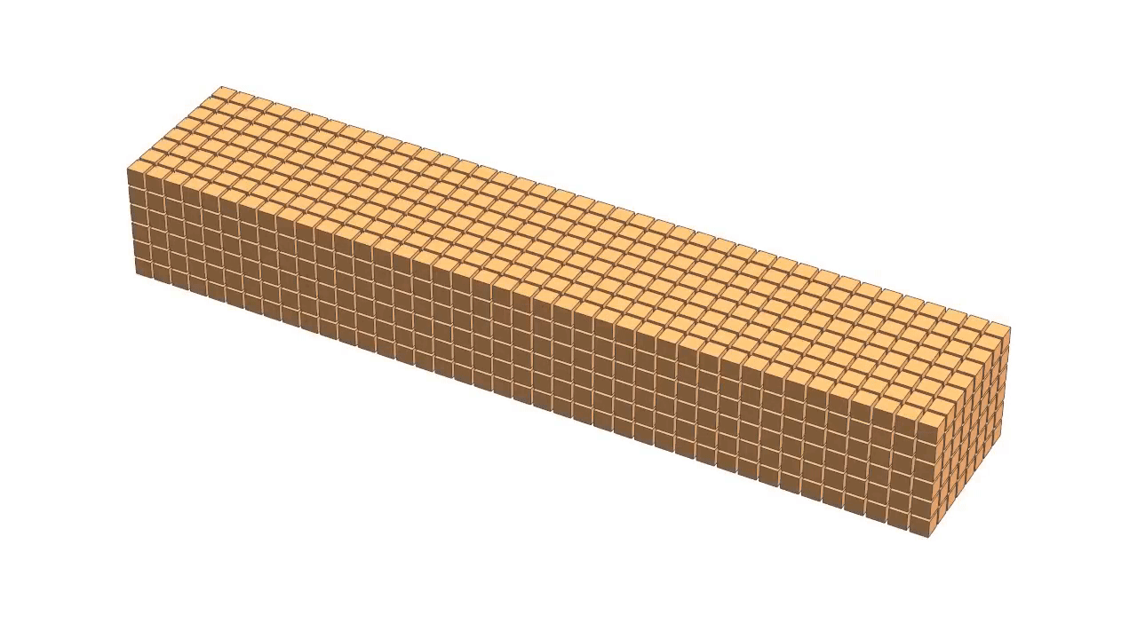Particle movement and direction of wave propagation of shear waves.² (click to play)

This cyclic movement can disrupt the soil structure and lead to gradual rearrangement of soil particles, leading to a reduction of pore space. For saturated soils, the pore space is filled with water. For the pore space to reduce under cyclic loading, the excessive pore water needs to drain from the pore space. If the loading happens fast - as it is the case for earthquake induce cyclic shearing - the excess pore water cannot drain freely. As a consequence the pore water pressure increases acting against the tendency of the soil to decrease in volume. Following the effective stress concept the increase in pore water pressure leads to a reduction of the effective stress. This reduction in effective stress is accompanied by a decrease in soil strength and stiffness. In the extreme case of vanishing mean effective pressure $p^\prime=0$ kPa a temporary transition of the soil from a solid to a liquid state occurs, a process known as liquefaction, see e.g. Soil behaviour under undrained cyclic shearing

Effects on geotechnical structures

The fundamental stability of geotechnical structures is intrinsically linked to the frictional properties of soils, specifically their capacity to resist shear stresses. When soils lose their shear strength or experience a substantial reduction in it, they are no longer capable of supporting the loads imposed by the weight of the structures. This loss of shear strength can precipitate structural failures, manifesting in various forms, including:

Compromised Foundation Stability: The loss of load-bearing capacity in foundations can result in excessive settlements or overturning of buildings. This is particularly critical in structures relying on the soil's shear strength for maintaining equilibrium and positional integrity.
Subsidence of Objects: Objects may sink into soils that have undergone liquefaction or significant strength reduction. This phenomenon is often observed in seismic events where the soil transitions into a fluid-like state, unable to support structural loads.
Surface Eruptions: The formation of sand volcanoes or mud extrusions on the surface, indicative of the upward movement of subsurface materials, is a direct consequence of soil liquefaction. This process can displace and redistribute soil particles, leading to the expulsion of materials at the ground surface.
Lateral Soil Movement under Dams: The lateral displacement of soil beneath dam structures can result in the formation of surface cracks and destabilization of the dam foundation. This phenomenon is of particular concern in seismic regions where shear wave-induced soil movements are prevalent.
Triggering of Landslides: A reduction in soil shear strength is a key factor in landslide initiation. The compromised soil can no longer support the overlying mass, leading to slope failures and mass movements.
Uplift of Underground Infrastructure: In cases where liquefied soil exerts upward pressure, underground infrastructure such as tunnels, pipelines or cables can be dislodged or uplifted, disrupting services and necessitating extensive repairs.

Understanding these failure mechanisms is essential for the design and construction of resilient geotechnical structures. It necessitates a comprehensive analysis of soil behavior under various loading conditions, particularly in seismically active regions. This understanding enables engineers to implement design strategies that mitigate the risks associated with the loss of soil shear strength, ensuring the safety and longevity of structures.

Uplift of Underground Infrastructure - A pen and paper example

To demonstrate the effect of soil liquefaction on the safety against uplift of underground structures, consider the following simple example of a tunnel embedded in a soil susceptible to liquefaction. The tunnel has a width of $b$ and a height defined as $h = z_b - z_t$. The key to ensuring the tunnel's stability lies in the balance of forces, specifically comparing the destabilizing vertical buoyancy forces $U$ against the cumulative stabilizing forces. These stabilizing forces consist of the tunnel's self-weight $W_T$, the (effective) weight of the soil above the tunnel $W_S$ (represented by the hatched area in the accompanying figure), and the tangential frictional forces $T$.

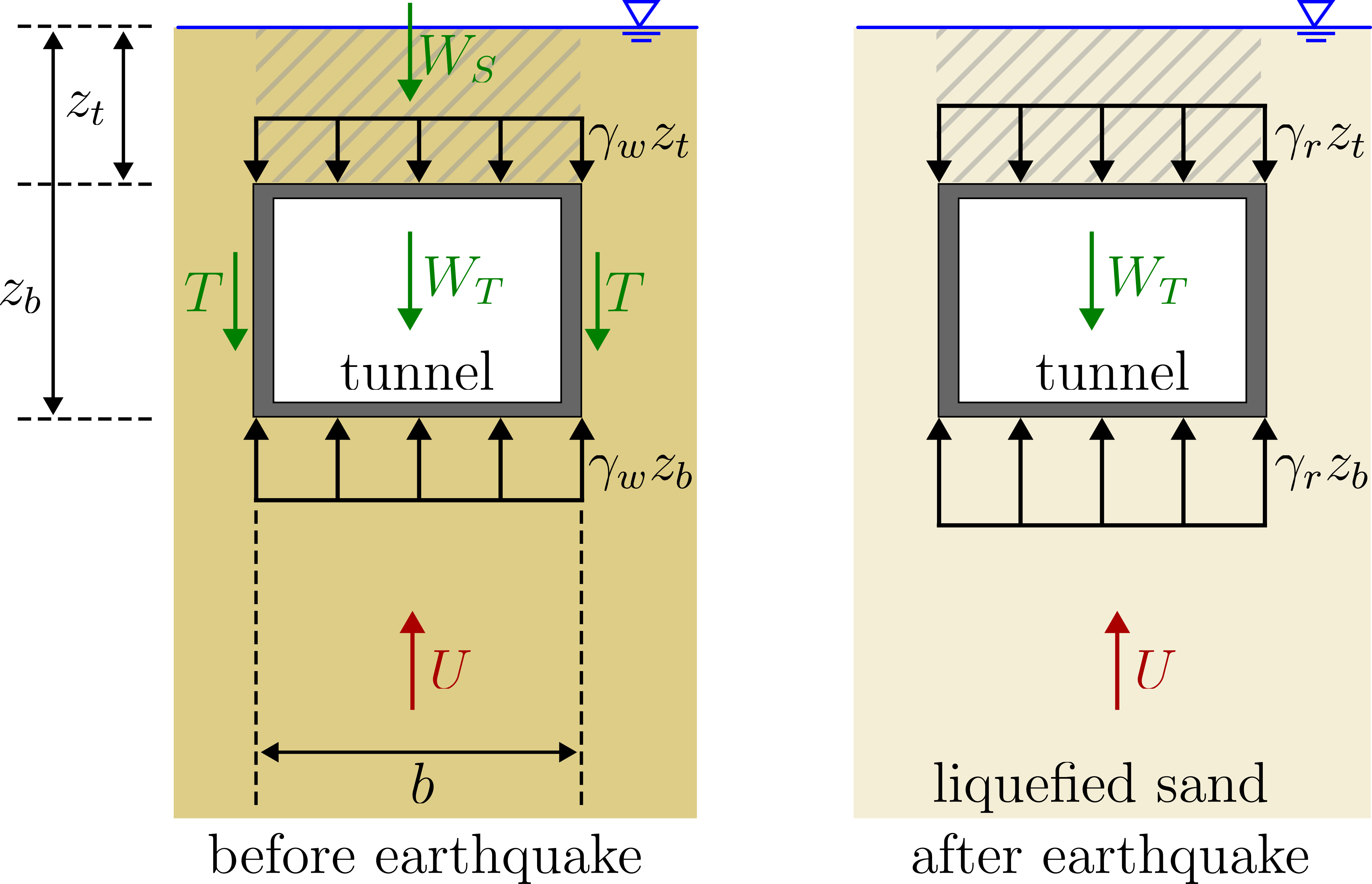
Uplift example: tunnel in liquefiable sand

Before the earthquake, the destabilizing forces are calculated as

\[ U = \gamma_w \left( z_b - z_t \right) b \]

where, $\gamma_w$, approximately 10 kN/m$^3$, represents the unit weight of water. The stabilizing forces $F_s$ are then determined as follows:

\[ F_s = W_T + W_S + 2T = W_T + \gamma^\prime b z_t + 2T \]

with the buoyancy weight of the soil $\gamma^\prime$.

After the earthquake - assuming complete liquefaction - the soil has no shear resistance anymore, thus $T^{liq}=0$. In addition, since the soil is fully liquefied, the buoyancy weight of the soil is $\gamma^\prime = 0$ kN/m$^3$, resulting in $W_S^{liq} = 0$. Consequently, the stabilizing forces after the earthquake, $F_s^{liq}$, are reduced to

\[ F_s^{liq} = W_T \]

Furthermore, the buoyancy force in the liquefied state, $U^{liq}$, has to be computed using the saturated weight $\gamma_r$ of the liquefied soil:

\[ U^{liq} = \gamma_r \left( z_b - z_t \right) b \]

With $\gamma_r$ approximately equal to $2\gamma_w$, the destabilizing forces are effectively doubled in comparison to the pre-earthquake state. Meanwhile, the stabilizing forces are significantly reduced due to the loss of shear strength and buoyancy weight in the soil. This drastic change in force dynamics leads to at least a halving of the safety margin against uplift for the tunnel structure.

This example highlights the critical importance of considering soil liquefaction in the design of underground structures, especially in seismically active regions. Methods for assessing the risk of liquefaction are discussed in the following section.

Assessment of liquefaction risk

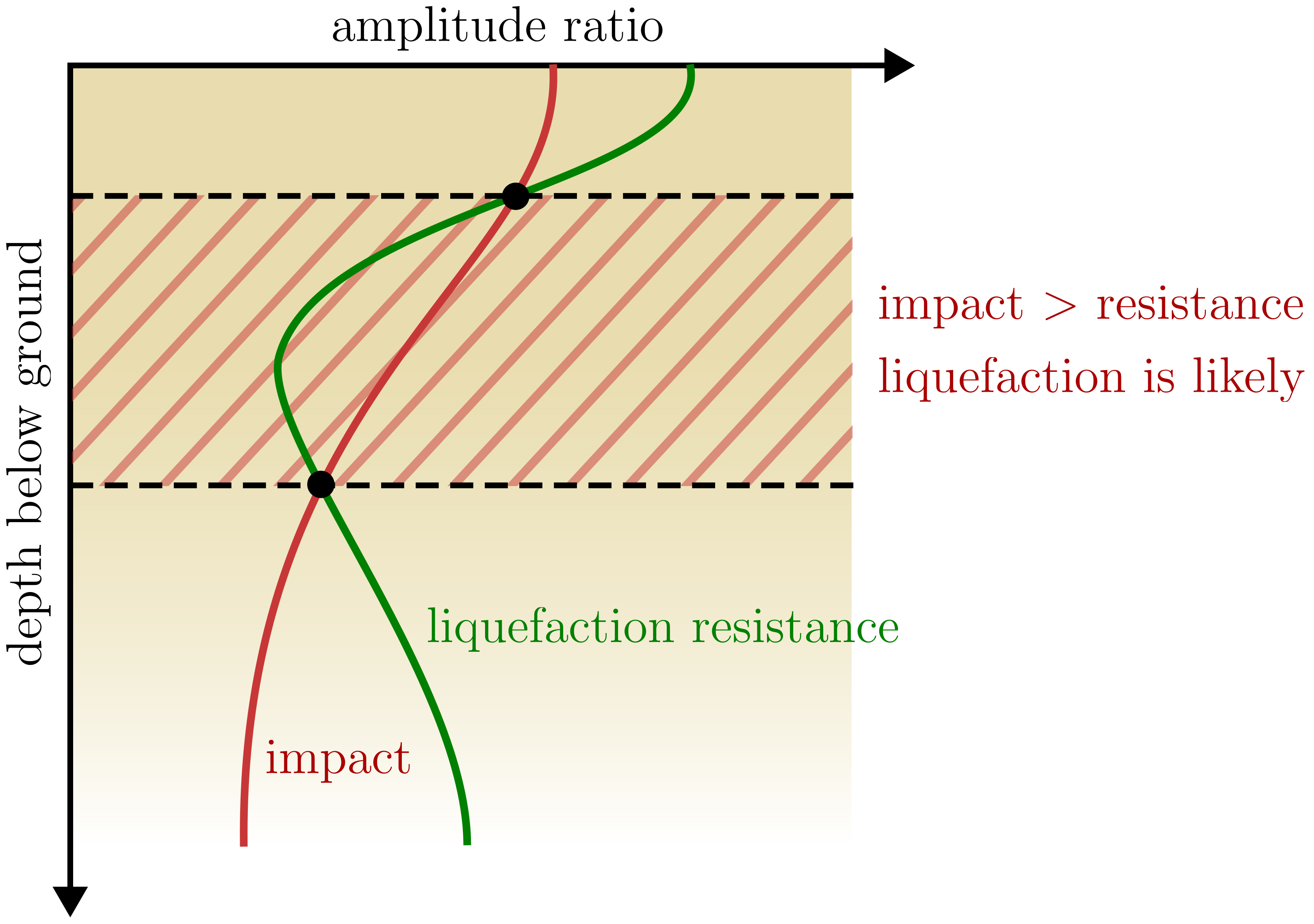
Assessing the risk of soil liquefaction is a challenging task, given the multitude of factors that influence this phenomenon. Fundamentally, if the seismic impact exceeds the soil's resistance to liquefaction, the likelihood of liquefaction increases. Determining these two critical components - impact and resistance - is essential in evaluating liquefaction risk.

Determining Seismic Impact:

Empirical Formulas: Commonly, the impact is estimated using empirical formulas that relate the expected seismic impact to the peak ground acceleration (PGA). PGA is derived from historical data and are region-specific, reflecting local seismic history and soil conditions.
Numerical Simulations: Another approach involves 1D wave propagation simulations using programs like SHAKE or EERA. Typically, these simulations employ simple non-linear elastic constitutive models. It's noteworthy that advanced versions of these programs can include pore water pressure accumulation, a vital factor in liquefaction assessment.

Determining Liquefaction Resistance:

Laboratory Tests: The resistance to liquefaction can be determined through undrained cyclic tests such as undrained cyclic triaxial tests on either undisturbed or reconstituted soil samples. The preparation of these samples is crucial and should represent the in situ soil formation history. This method allows for a controlled and detailed understanding of (the specific) soil behavior under seismic loading.
Field Tests: A widely adopted method involves correlating liquefaction resistance with probing resistances, such as the corrected blow count $N_{(60)}$ of Standard Penetration Tests (SPT) or the cone tip resistance of Cone Penetration Tests (CPT). Additionally, correlations with shear wave velocity exist. However, it's important to acknowledge the inherent uncertainties and limitations in extrapolating field test results to predict liquefaction behavior.

Advancements in Computational Techniques:

With the advent of increased computational power and specialized software, a more integrated approach to assessing liquefaction hazards has emerged. Advanced constitutive models and numerical methods considering the accumulation of pore water pressure during seismic loading allow for a comprehensive assessment within a single calculation. Such simulations can be applied in 1D, 2D, or 3D representations of the real system, offering a more nuanced and realistic simulation of soil behavior under seismic conditions but requires careful calibration based on laboratory tests and validation against field observations. More information on this topic is given in the lecture Numerical Simulations in Geotechnical Engineering taking place in the summer semester.

Impact from empirical formulas with peak ground acceleration (PGA)

A widely used formula for estimating the impact of earthquakes in terms of the cyclic stress ratio (CSR) is the one developed by Seed and Idriss in 1971³:

Seed and Idriss, 1971³

\[ CSR_{7.5} = 0.65 \left( \dfrac{\sigma_v}{\sigma_v^\prime} \right) \left( \dfrac{a_{max}}{g}\right) r_d \]

The Eurocode proposes a slightly different formula:

\[ CSR_{7.5} = 0.65 \left( \dfrac{\sigma_v}{\sigma_v^\prime} \right) \left( \dfrac{a_{max}}{g}\right) S \]

where:

$CSR_{7.5}$ represents the cyclic stress ratio for an earthquake of magnitude 7.5, serving as a standard reference point.
$\sigma_v$ is the total overburden pressure at the depth considered.
$\sigma_v^\prime$ denotes the effective overburden pressure at the same depth.
$a_{max}$ is the maximum horizontal acceleration at the ground surface.
$g$ symbolizes the acceleration due to earth’s gravity.
$r_d$ is the stress reduction factor, which accounts for the influence of depth and soil conditions on seismic response.
Currently, there are no specific charts or formulas for determining $S$, so it is often assumed that $S = r_d$.

Derivation

Above equation can be derived a rigid soil body subjected to horizontal acceleration as displayed in below figure.

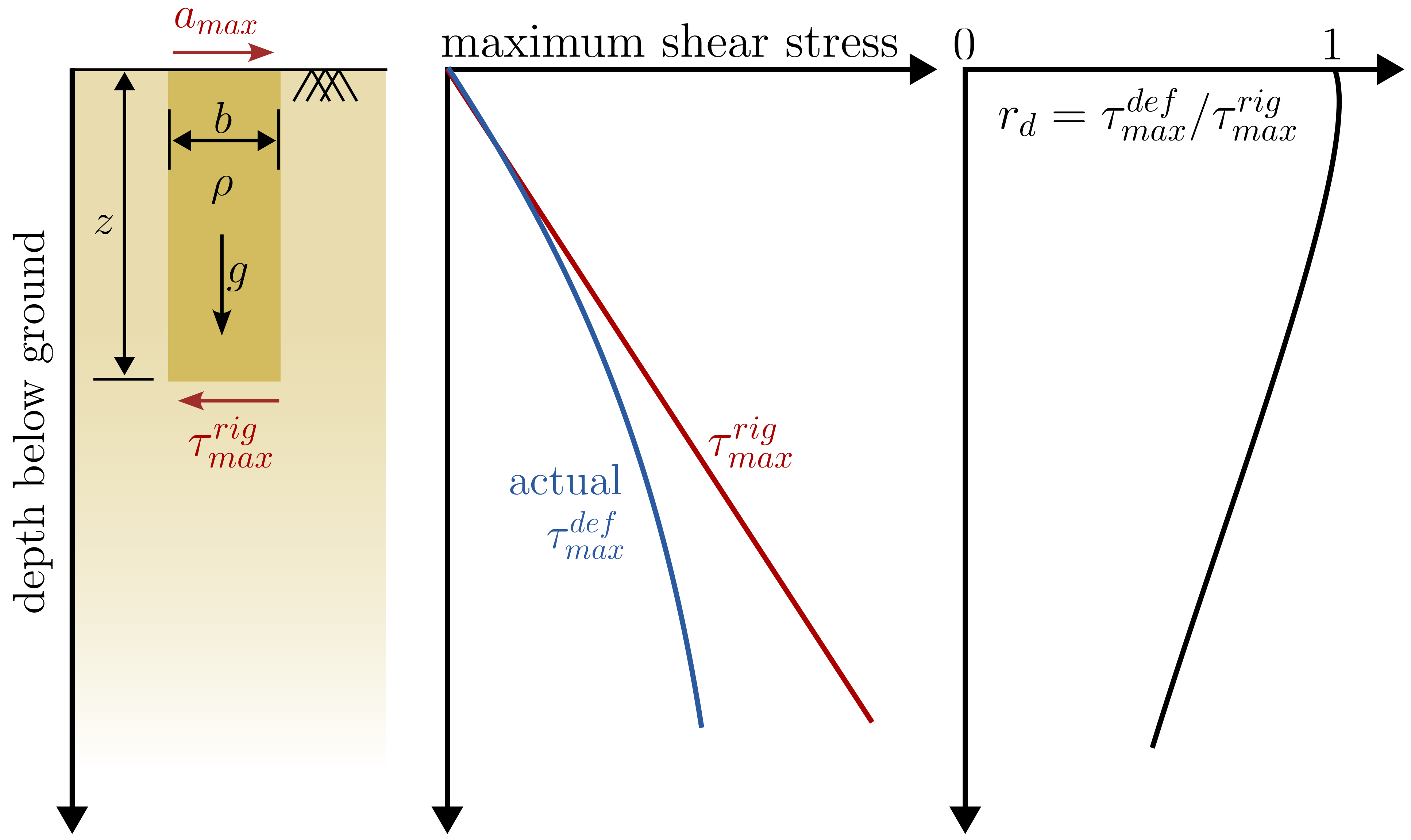
Rigid soil body analogy for the derivation of the Seed and Idris equation.

In this case, the maximum shear force at the base of the rigid soil body $\tau_{max}^{rigid}$ can be calculated as follows

\[ \begin{aligned} \tau_{max}^{rigid} &= \dfrac{m \cdot a_{max}}{b \cdot 1} = \dfrac{\rho \cdot z \cdot b \cdot 1 \cdot a_{max}}{b \cdot 1} = \dfrac{\gamma \cdot z \cdot a_{max}}{g} \\ & = \sigma^\prime_v(z) \dfrac{a_{max}}{g} \end{aligned} \]

According to above equation $\tau_{max}^{rigid}$ increases linearly with depth. In reality, however, the soil column is deformable and does not behave as a rigid body. The actual shear stress $\tau_{max}^{def}$ would be less than $\tau_{max}^{rigid}$ (see right-hand side of above figure). To account for situation, the stress distribution factor is introduced in the equation:

\[ \tau_{max} = \sigma^\prime_v(z) \dfrac{a_{max}}{g} r_d ~~~\text{with:}~~ r_d = \dfrac{\tau_{max}^{def}}{\tau_{max}^{rigid}} < 1 \]

Seismic loading on soil produces irregular shear stress histories. To approximate the equivalent uniform shear stress $\tau_{av}$, empirical evidence suggests that it is about 65 % of the maximum shear stress³.

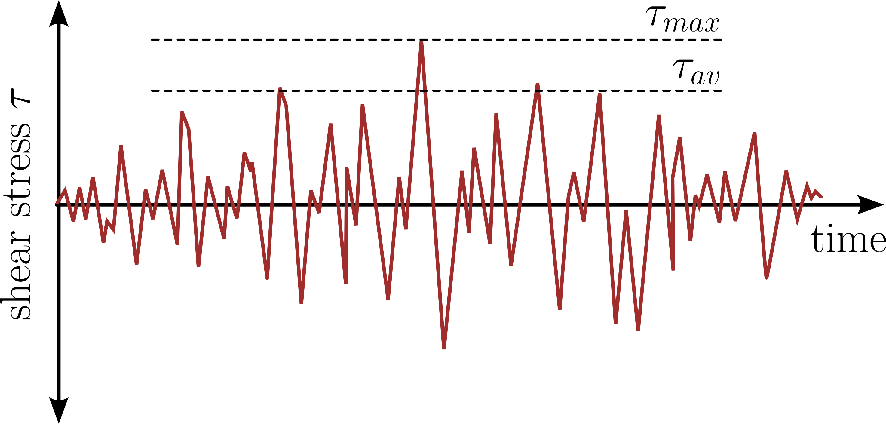
Exemplary time history of shear stress during an earthquake, modified from ³

Thus, the average cyclic shear stress is estimated as:

\[ \tau_{av} = 0.65~ \sigma^\prime_v(z) \dfrac{a_{max}}{g} r_d \]

Finally, the CSR is obtained by normalizing $\tau_{max}$ with the total overburden pressure:

\[ CSR = \dfrac{\tau_{av}}{\sigma_v} = 0.65~ \dfrac{\sigma^\prime_v(z)}{\sigma_v} \dfrac{a_{max}}{g} r_d \]

It's important to recognize the inherent assumptions in this model, including the variability of $r_d$ and the empirical nature of the 65 % approximation.

Stress distribution factor $r_d$

Seed and Idris (1970)³ provide the results from computations of the value of $r_d$ for a wide variety of earthquake motions and soil conditions having sand in the upper 15 m, showing that $r_d$ falls within the range of $r_d \leq 0.3 \leq 1.0$ as shown in below figure. It may be seen that up to approximately 10 m depth the scatter of the results is not great and for any of the deposits, the error involved in using the average values shown by the dashed line would generally be less than about 5 %.

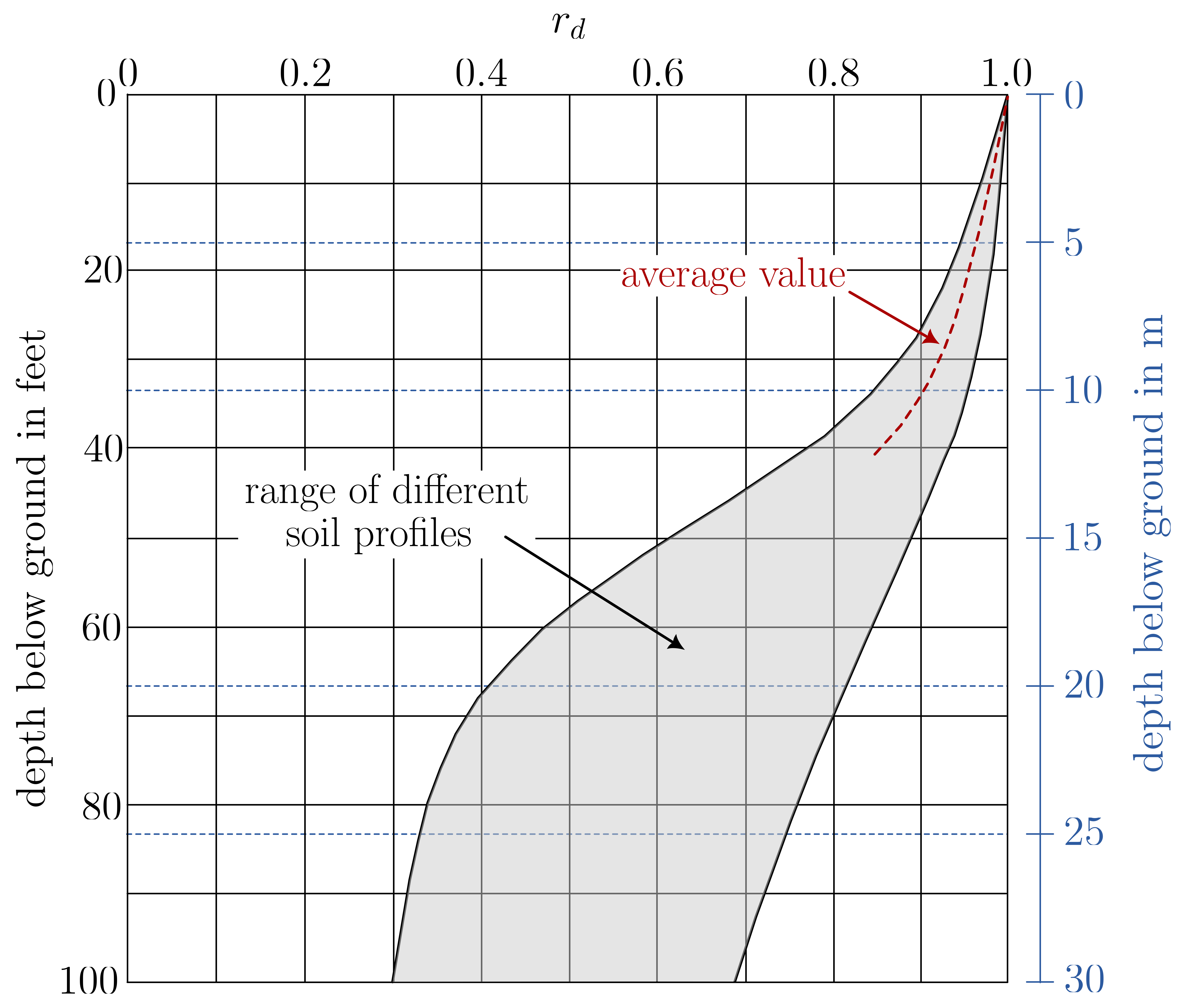
Range of values of $r_d$ for different soil profile, modified from ³

Different relations for $r_d$ have been proposed in the past, some popular ones are listed in the table below.

Method	$r_d$
Kayen et al (1992)	$1 - 0.012z$
Idris (NCEER 1997)	$1 - 0.00765 z$ for $z \leq 9.15$ m $1.174 - 0.0267 z$ for $9.15 < z \leq 23$ m $0.744 - 0.008 z$ for $23 < z \leq 30$ m $0.5$ for $z > 30$ m
Blake (1996)	$\dfrac{1.0-0.4113 z^{0,5}+0.04052z+0.001753z^{1,5}}{1.0-0.4177z^{0.5}+0.05729z-0.006205^{1.5}+0,00121z^{2}}$
Idriss & Boulanger (2010)	$r_{d}=e x p(\alpha(z)+\beta(z)\cdot M_{w})$ $\alpha(z)=-1.012-1.126\cdot\mathrm{sin}\left({\frac{z}{11.73}}+5.133\right)$ $\beta(z)=0.106-0.118\cdot\sin\left({\frac{z}{11.28}}+5.142\right)$

Magnitude Scaling Factor (MSF)

It is important to note that the above formulas are calibrated for an earthquake of magnitude 7.5. To adjust the CSR value for earthquakes of different magnitudes, a Magnitude Scaling Factor (MSF) should be applied to $CSR_{7.5}$. Several methods have been proposed for calculating the MSF:

Method	MSF
Tokimatsu & Seed (1987)	$2.5-0.2M$
Idris (NCEER 1997)	$(7.5/M)^{2.56}$
Idriss & Boulanger (2008)	$6.9 e^{-M/4}-0.058 < 1.8$
Idriss & Boulanger (2014)	$1+(MSF_{max}-1)\left(8.64 e^{-M/4}-1.325\right)$ $MSF_{max}=1.09+\left(N_{1,60}c_s / 31.5 \right)^2 < 2.2$

Concluding remark

Caution

The procedure described above is relatively easy to apply in practice. However, the many relationships for the different factors ($r_d$, $MSF$) and the simplified estimation of $\tau_{av}$ should make it clear that it has large inherent uncertainties. When using it, it should always be checked whether there are regional / site-specific empirical values (different from above estimates) that can be used instead of - or in addition to - the common estimates from the literature.

Resistance

In general the liquefaction resistance can be estimated based on laboratory test series or by field tests such as Standard Penetration Tests (SPT) or Cone Penetration Tests (CPT). Whilst site-specific material is used to generate resistance curves from laboratory tests, the estimation of liquefaction resistance from field tests is based on a comparison with correlations documented in the literature. The different methods are briefly discussed in the following sections.

Resistance from laboratory tests

The basis for the evaluation of the liquefaction resistance based on laboratory tests is the relationship between the amplitude ratio CSR and the number of cycles to liquefaction derived in Section Cyclic stress ratio. A typical example of such a relation is depicted in the following figure.

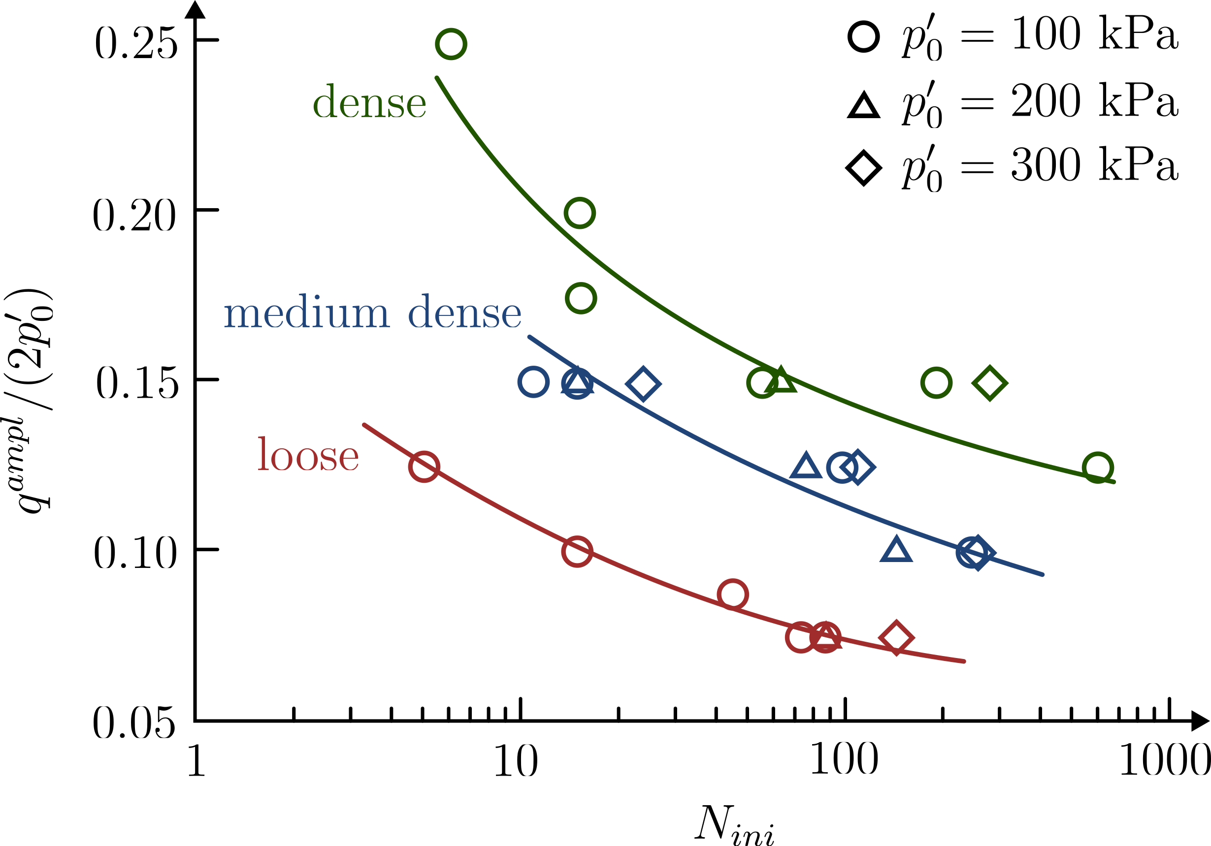
Amplitude-stress ratio versus number of cycles to initial liquefaction from undrained cyclic triaxial tests on loose, medium dense and dense Karlsruhe Finesand

The soil is considered successible for liquefaction if the $CSR$ of the earthquake $CSR^{eq}$ is larger than the $CSR^{lab}$ obtained from the laboratory tests

However, the CSR-$N_{ini}$ graph shows clearly that the resistance of sand against liquefaction depends on the number of stress cycles during an expected earthquake. $CSR^{lab}$ must thus be evaluated at the same number of cycles from the design earthquake $N^{eq}$. The first step is to determine $CSR^{eq}$ from the earthquake as described in above Section. Determining the number of cycles from the design earthquake signal that corresponds to the determined $CSR^{eq}$ remains an open issue. How to do this for a real, irregular earthquake signal is not obvious. Seed and Idriss (1982)⁴ proposed to replace an irregular time history of earthquake loading by an equivalent stress history with a constant amplitude as shown below.

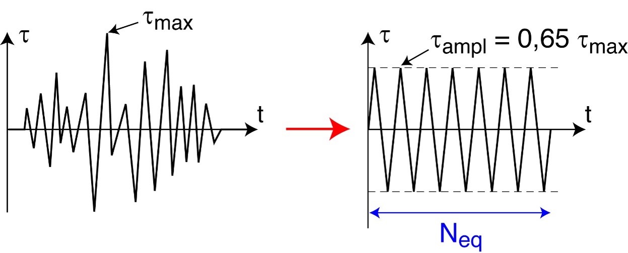
Transformation of an irregular shear stress time history to an equivalent stress history with constant amplitude

Following this approach, Seed and Idriss (1982)⁴ proposed the following (rough!) estimate of $N^{eq}$

Richter scale of earthquake magnitude (M)	Equivalent number of stress cycles $N^{eq}$ (rough estimate.)
8.5	26
7.5	15
6.75	10
6	5-6
5.25	2-3

With above estimates of $N^{eq}$ the number of cycles changing with the earthquake magnitude is taken into account by reducing the soil resistance for quakes of greater magnitude:

When an earthquake includes only a few cycles (a case of smaller earthquake magnitude), the soil can resist a greater stress ratio.
In contrast, when the expected number of cycles is large (an earthquake of larger magnitude), the soil can resist a smaller stress ratio.

This is exemplarily illustrated for two magnitudes $M_1 > M_2$ in below figure.

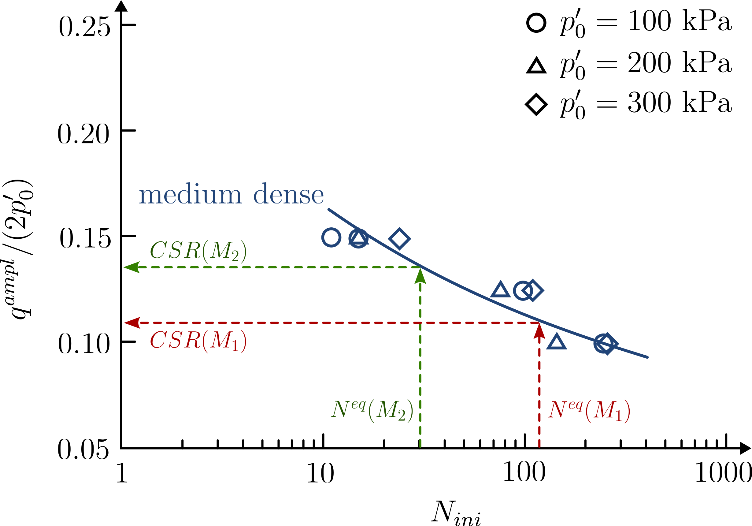
If the so obtained CSR are larger than $CSR^{eq}$, the soil is not considered to be at risk of liquefaction (under the given load!).

Warning

Since soil behaviour under (undrained) cyclic loading is highly sensitive to its state (density, stress, structure, ...) care must be taken when performing the cyclic tests forming the basis of the $N-CSR$ curves used to evaluate the liquefaction resistance. If possible, undisturbed samples should be used (e.g. frozen soil samples). If not possible, disturbed samples should be prepared to reflect in situ soil formation as closely as possible.

Resistance from SPT correlations (SPT)

Seed and Idriss (1982)⁴ conducted a comprehensive study to understand the relationship between the CSR and Standard Penetration Test values (SPT-N), at various sites that either experienced or did not experience signs of liquefaction during past seismic events. Their primary objective was to investigate the onset of liquefaction in relation to the SPT-N values. Their results are plotted in terms of $CSR$ over modified values of SPT-N$_1$, referred to as $N^{SPT,mod}_1$ from here on. In this representation, sites that displayed signs of liquefaction are marked with solid black circles, while those that did not are indicated with hollow circles.

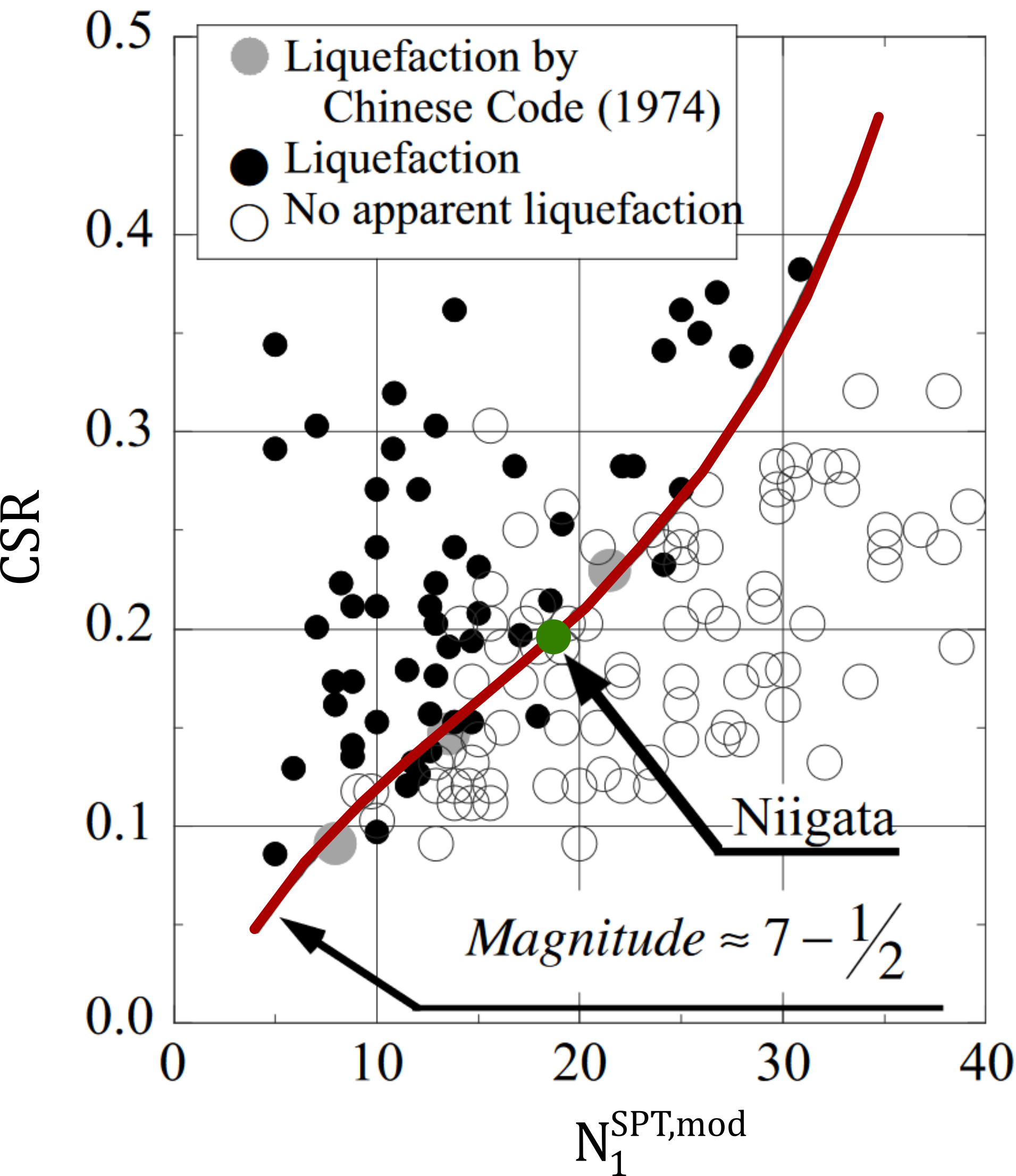
Seismic stress ratio produced by earthquakes of magnitude = 7.5 at sites with and without liquefaction, modified from ⁴

$N^{SPT,mod}_1$ (often denoted as $(N_1)_{60}$) is the number of blows measured in situ before the earthquake related to an overburden stress of 100 kPa, using the following formula:

\[ N^{SPT,mod}_1 = \frac{1.7}{\left[\frac{\sigma'_v (\text{kPa})}{98}\right]+0.7} N \]

Although this method is not highly precise, the results effectively delineate a boundary, highlighted in red in the figure above, between the data points from sites that liquefied and those that did not. This boundary indicates the liquefaction resistance of sand and its correlation with $N^{SPT,mod}_1$. If a data point lies above this trend line, the likelihood of liquefaction is high; if below, liquefaction is considered unlikely.

Notice that fines content $FC$ in sandy soil reduces the measured SPT-N value. To account for this, there are several empirical corrections. Seed (1987)⁵ proposed to increase $N^{SPT,mod}_1$ the observed by a specific increment $\Delta N$ to account for the influence of fine content.

\[ (N^{SPT,mod}_1)_{observed} = (N^{SPT,mod}_1)_{measured} + \Delta N \]

where:

FC (%)	$\Delta N$
10	1
25	2
50	4
75	5

Validity

It should be noted that this diagram is valid for earthquake magnitude of 7.5 for which the number of cycles is about 15. For $N^{SPT,mod}_1 < 15$ soil is considered to have a possibility of liquefaction⁶.

Resistance from Cone Penetration Tests (CPT)

Amongst others, Boulanger and Idriss (2014)⁷ proposed a correlation between the tip resistance from Cone Penetration Tests (CPT) and the CSR. The procedure is analogous to the SPT-N correlation discussed above, with similar benefits and limitations. The correlation as well as the underlying data is illustrated in the figure below.

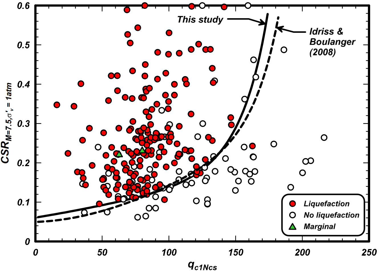
CPT case history database of liquefaction in cohesionless soils with various fines contents in terms of equivalent CSR for $M = 7.5$ and equivalent clean sand $q_{c1Ncs}$ ⁷

Therein $q_{c1Ncs}$ is the overburden-stress and fine content corrected cone tip resistance $q_c$:

\[ q_{c1Ncs} = q_c\frac{1.7}{\left[\frac{\sigma'_v (\text{kPa})}{100}\right]+0.7} + \Delta q_{Ncs} \]

where $q_{Ncs}$ is the correction to account for the fines content (FC) and is defined as follows:

\[ \Delta q_{Ncs} = \left[ 11.9 + \frac{q_{c1N}}{14.6} \right] \exp \left( 1.63 - \frac{9.7}{FC + 2} - \left( \frac{15.7}{FC + 2} \right)^2 \right) \]

The trend line indicating the liquefaction resistance, here denoted as CRR, is given by the following equation:

\[ CRR_{M=7.5, \sigma'_v=100\text{kPa}} = \exp \left( \frac{q_{c1Ncs}}{113} + \left( \frac{q_{c1Ncs}}{1000} \right)^2 - \left( \frac{q_{c1Ncs}}{140} \right)^3 + \left( \frac{q_{c1Ncs}}{137} \right)^4 \right) - 2.8 \]

Concluding remarks

At this point it should be clear that the assessment of the liquefaction risk of soils is characterised by large uncertainties due to the many influencing factors and the (mathematically) complex soil behaviour under (undrained) cyclic loading.

Simple, practical methods for estimating the liquefaction risk were presented. Their underlying data base, challenges and inherent uncertainties are discussed. Careful application of these methods is required. It is recommended to combine several of these methods to obtain a more comprehensive picture of the liquefaction risk and the uncertainties of the assessment. Complementary numerical simulations are recommended, but are beyond the scope of this presentation.

https://de.wikipedia.org/wiki/Liste_von_Erdbeben_in_Deutschland ↩
Animation created with Mathematica following https://blog.wolfram.com/2011/03/18/built-to-last-understanding-earthquake-engineering/ ↩
H. B. Seed and I. M. Idriss, ‘A Simplified Procedure for Evaluating Soil Liquefaction Potential.’, California Univ., Berkeley. Earthquake Engineering Research Center., PB198009, 1970. Accessed: Dec. 20, 2023. [Online]. Available: https://ntrl.ntis.gov/NTRL/dashboard/searchResults/titleDetail/PB198009.xhtml ↩↩↩↩
H. B. Seed and I. M. Idriss, Ground motions and soil liquefaction during earthquakes. in Engineering monographs on earthquake criteria, structural design, and strong motion records, no. v. 5. Berkeley, Calif: Earthquake Engineering Research Institute, 1982. ↩↩↩
Seed, H.B. (1987) Design problems in soil liquefaction, J. Geotech. Eng., Vol. 113, No. 8, pp. 827–845. ↩
I. Towhata, Geotechnical earthquake engineering. in Springer series in geomechanics and geoengineering. Berlin: Springer-Verlag, 2008. ↩
R. W. Boulanger and I. Idriss, ‘CPT and SPT based liquefaction triggering procedures’, Report No. UCD/CGM.-14, vol. 1, 2014. ↩

Method	\(r_d\)
Kayen et al (1992)	\(1 - 0.012z\)
Idris (NCEER 1997)	\(1 - 0.00765 z\) for \(z \leq 9.15\) m \(1.174 - 0.0267 z\) for \(9.15 < z \leq 23\) m \(0.744 - 0.008 z\) for \(23 < z \leq 30\) m \(0.5\) for \(z > 30\) m
Blake (1996)	\(\dfrac{1.0-0.4113 z^{0,5}+0.04052z+0.001753z^{1,5}}{1.0-0.4177z^{0.5}+0.05729z-0.006205^{1.5}+0,00121z^{2}}\)
Idriss & Boulanger (2010)	\(r_{d}=e x p(\alpha(z)+\beta(z)\cdot M_{w})\) \(\alpha(z)=-1.012-1.126\cdot\mathrm{sin}\left({\frac{z}{11.73}}+5.133\right)\) \(\beta(z)=0.106-0.118\cdot\sin\left({\frac{z}{11.28}}+5.142\right)\)

Method	MSF
Tokimatsu & Seed (1987)	\(2.5-0.2M\)
Idris (NCEER 1997)	\((7.5/M)^{2.56}\)
Idriss & Boulanger (2008)	\(6.9 e^{-M/4}-0.058 < 1.8\)
Idriss & Boulanger (2014)	\(1+(MSF_{max}-1)\left(8.64 e^{-M/4}-1.325\right)\) \(MSF_{max}=1.09+\left(N_{1,60}c_s / 31.5 \right)^2 < 2.2\)

FC (%)	\(\Delta N\)
10	1
25	2
50	4
75	5