Simplified stress conditions

In the realm of geotechnical engineering, the behavior of soils and rocks under different stress states is of paramount importance. Engineers often find themselves analyzing massive bodies of soil, such as dams, embankments, or expansive natural terrain. Given the vastness of these bodies and the complexities inherent in three-dimensional stress analysis, a simplification is often sought. This is where the concepts of plane strain or axisymmetry come into play.

Plane strain conditions

"Plane strain" is a term used to describe a specific state of deformation where displacements in one direction (usually the out-of-plane direction) are zero. In essence, the strain components associated with this direction are nil. This implies that the stresses and strains in that direction remain constant along its entire length. One could visualize plane strain as a condition where an infinitely long body experiences deformation in a two-dimensional plane, while its third dimension remains unaffected.

In geotechnical contexts, plane strain conditions are frequently assumed for problems where one dimension is very large compared to the other two. For instance, in the analysis of an infinitely long dam or retaining wall, the length along the dam's or wall's axis is much larger than its depth or thickness. Thus, the effects due to this extensive dimension can be considered constant, allowing engineers to focus their analysis on a 2D cross-section. A typical example for a geotechnical structure suitable for plane strain simplification are embankments as depicted below.

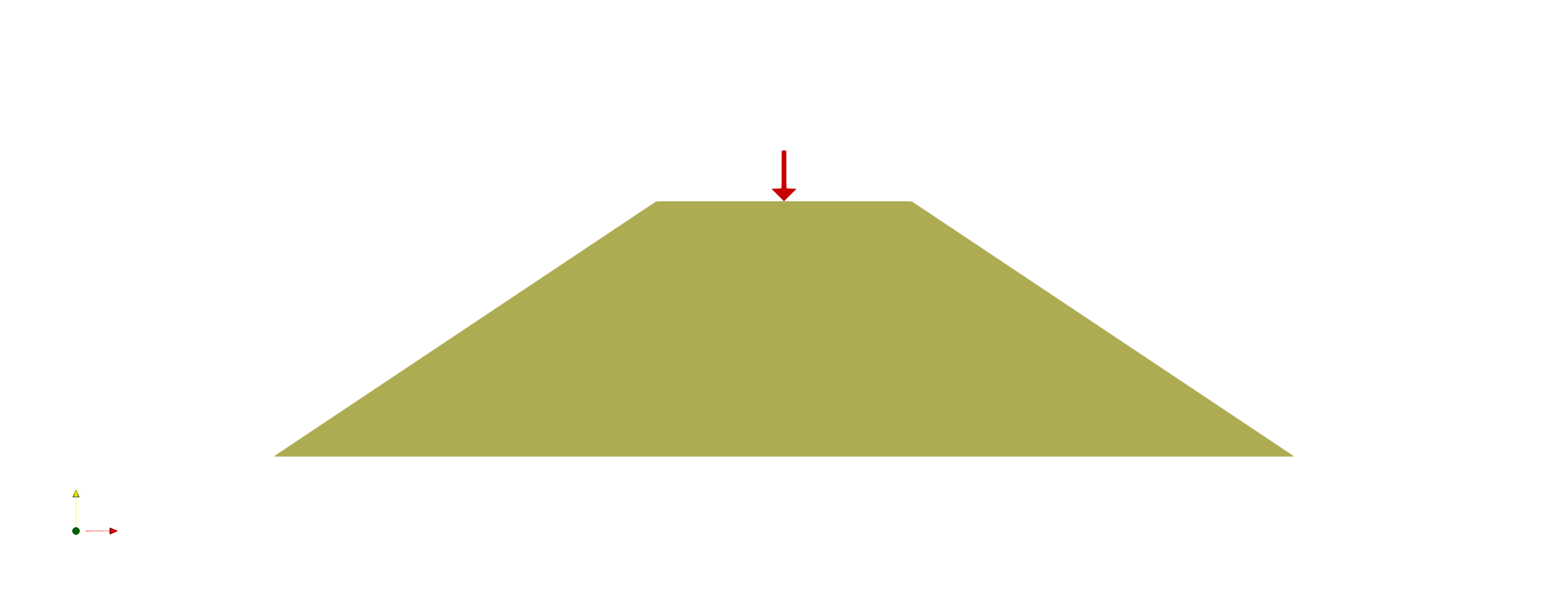Typical example of a geotechnical structure often suitable for a simplification to a plane strain problem (click to play)

In three dimensions, the general form of the stress tensor \(\boldsymbol{\sigma}\) and strain tensor \(\boldsymbol{\varepsilon}\) can be represented as:

\[ \boldsymbol{\sigma} = \begin{bmatrix} \sigma_{xx} & \sigma_{xy} & \sigma_{xz} \\ \sigma_{yx} & \sigma_{yy} & \sigma_{yz} \\ \sigma_{zx} & \sigma_{zy} & \sigma_{zz} \\ \end{bmatrix} ~~~\text{and}~~~ \boldsymbol{\varepsilon} = \begin{bmatrix} \varepsilon_{xx} & \varepsilon_{xy} & \varepsilon_{xz} \\ \varepsilon_{yx} & \varepsilon_{yy} & \varepsilon_{yz} \\ \varepsilon_{zx} & \varepsilon_{zy} & \varepsilon_{zz} \\ \end{bmatrix} \]

For plane strain, the condition implies no strain in one of the planes, here chosen to be the z-direction. This means:

\[ \varepsilon_{zz} = 0~~~,~~~ \varepsilon_{xz} = 0 ~~~,~~~ \varepsilon_{yz} = 0 \]

This simplification means that the strain occurs only within the \(x-y\) plane and not in the out-of-plane \(z\)-direction.

Consequently, our strain tensor becomes:

\[ \boldsymbol{\varepsilon} = \begin{bmatrix} \varepsilon_{xx} & \varepsilon_{xy} & 0 \\ \varepsilon_{yx} & \varepsilon_{yy} & 0 \\ 0 & 0 & 0 \\ \end{bmatrix} \]

For stresses, in the context of plane strain, we don't assume that stresses in the \(z\)-direction are zero. However, due to equilibrium and compatibility, the stress tensor for plane strain usually takes the form:

\[ \boldsymbol{\sigma} = \begin{bmatrix} \sigma_{xx} & \sigma_{xy} & 0 \\ \sigma_{yx} & \sigma_{yy} & 0 \\ 0 & 0 & \sigma_{zz} \\ \end{bmatrix} \]

Where: \(\sigma_{zz}\) is not necessarily zero but might be a function of \(\sigma_{xx}\) and \(\sigma_{yy}\), depending on the constitutive model emplyed.

Although very usefull and often applied, it's crucial to understand the limits of this simplification. Plane strain is a specific state of stress and deformation, and its assumption is only valid under certain conditions. They key assumptions of the plane strain simplification not only apply to the geotechnical structure but to the ground conditions and loading conditions as well. Careful judgement is required and the implications of the plane strain representation need to be understood. An illustrative example of the effect of plane strain simplifications is given in (Lees 2016)¹ and depicted in the following.

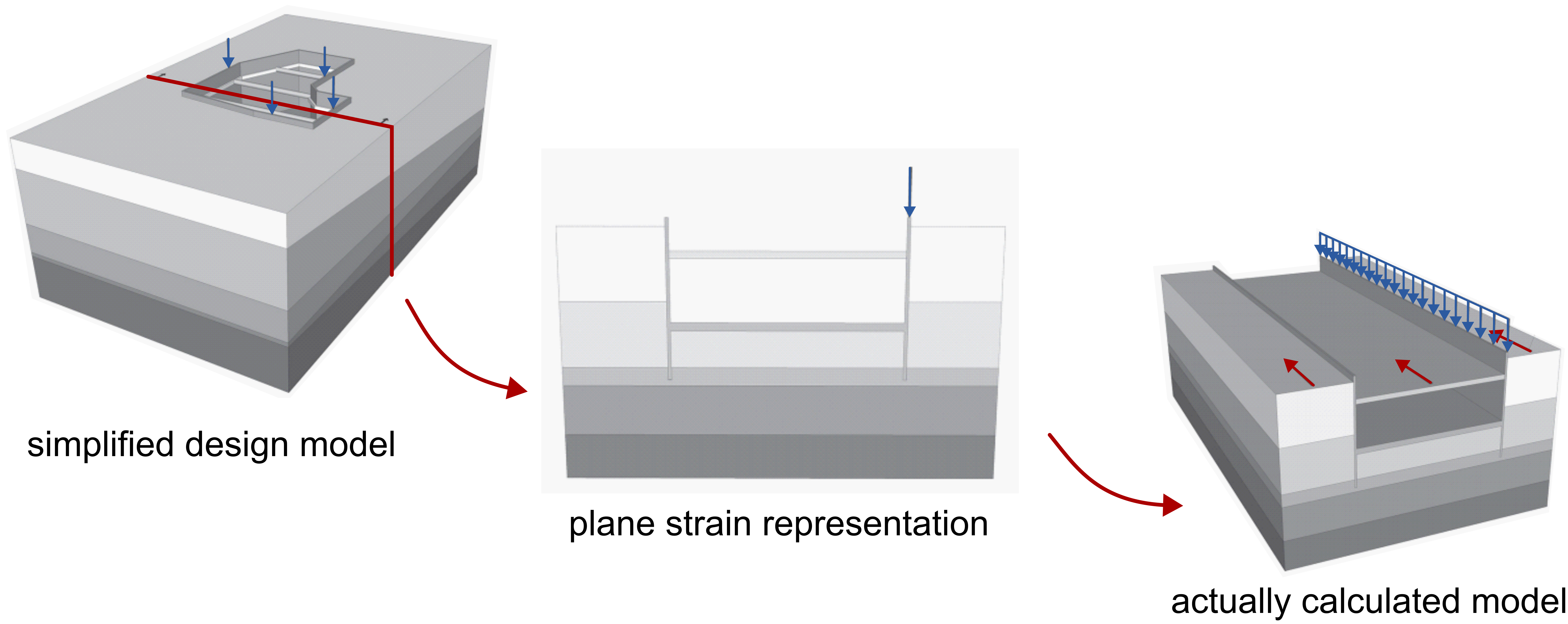plane-strain-example Example of the implications of plane strain simplifications, adapted from ¹

Axisymmetric conditions

In geotechnical engineering, many problems encountered are inherently symmetrical about an axis, such as the load distribution around piles, the stress distribution beneath circular footings, or the stresses in a cylindrical tunnel lining. For such problems, an axisymmetric analysis can be employed, which simplifies the problem by assuming that all variables are symmetric with respect to a central axis, typically denoted as the \(z\) axis. For such problems, axisymmetric simplification reduces the problem to a 2D plane while still accounting for three-dimensional effects.

For axisymmetric problems, we consider a cylindrical coordinate system \((r, \theta, z)\), where \(r\) is the radial distance from the central axis, \(\theta\) is the angular coordinate, and \(z\) is the axial coordinate (along the axis of symmetry). In axisymmetric problems, any variable is independent of \(\theta\). The stress and strain components that are functions of \(\theta\) go to zero, which leads to the simplification of the tensors.

The transformation is as follows:

\(\sigma_{xx}\) becomes \(\sigma_{rr}\) (radial stress)
\(\sigma_{yy}\) becomes \(\sigma_{\theta\theta}\) (hoop or circumferential stress)
\(\sigma_{zz}\) remains \(\sigma_{zz}\) (axial stress)

A similar transformation holds for strain. The general form of the stress and strain tensors in three dimensions in cylindical coordinates is:

\[ \boldsymbol{\sigma} = \begin{bmatrix} \sigma_{rr} & \sigma_{r\theta} & \sigma_{rz} \\ \sigma_{\theta r} & \sigma_{\theta\theta} & \sigma_{\theta z} \\ \sigma_{zr} & \sigma_{z\theta} & \sigma_{zz} \\ \end{bmatrix} ~~~\text{and}~~~ \boldsymbol{\varepsilon} = \begin{bmatrix} \varepsilon_{rr} & \varepsilon_{r\theta} & \varepsilon_{rz} \\ \varepsilon_{\theta r} & \varepsilon_{\theta\theta} & \varepsilon_{\theta z} \\ \varepsilon_{zr} & \varepsilon_{z\theta} & \varepsilon_{zz} \\ \end{bmatrix} \]

Therein, \(\sigma_{rr}\), \(\sigma_{\theta\theta}\), and \(\sigma_{zz}\) are the normal stresses. The off-diagonal elements represent the shear stresses.

For axisymmetric conditions, the assumption is that any variable does not vary in the \(\theta\) direction. As a result:

Shear stresses which involve the \(\theta\) component are zero:
\(\sigma_{r\theta} = \sigma_{\theta r} = \sigma_{\theta z} = \sigma_{z\theta} = 0\)
Similarly, the corresponding strain components are also zero:
\(\varepsilon_{r\theta} = \varepsilon_{\theta r} = \varepsilon_{\theta z} = \varepsilon_{z\theta} = 0\)

Thus, the simplified stress tensor for axisymmetric conditions becomes:

\[ \boldsymbol{\sigma} = \begin{bmatrix} \sigma_{rr} & 0 & \sigma_{rz} \\ 0 & \sigma_{\theta\theta} & 0 \\ \sigma_{zr} & 0 & \sigma_{zz} \\ \end{bmatrix} ~~~\text{and}~~~ \boldsymbol{\varepsilon} = \begin{bmatrix} \varepsilon_{rr} & 0 & \varepsilon_{rz} \\ 0 & \varepsilon_{\theta\theta} & 0 \\ \varepsilon_{zr} & 0 & \varepsilon_{zz} \\ \end{bmatrix} \]

Notice that in axisymmetric conditions, the circumferential strain \(\varepsilon_{\theta\theta}\) is related to the radial strain due to the constraint of no change in circumference, giving rise to the relation:

\[ \varepsilon_{\theta\theta} = -\varepsilon_{rr}, \]

which is a direct result of the axisymmetric assumption and the continuity of the material in the circumferential direction.

Triaxial conditions

Triaxial conditions, often encountered in geotechnical testing procedures like the triaxial shear test, assume a specific simplified state of stress and strain. The objective of such tests is to measure the strength and deformation characteristics of soils under controlled drainage and confinement conditions.

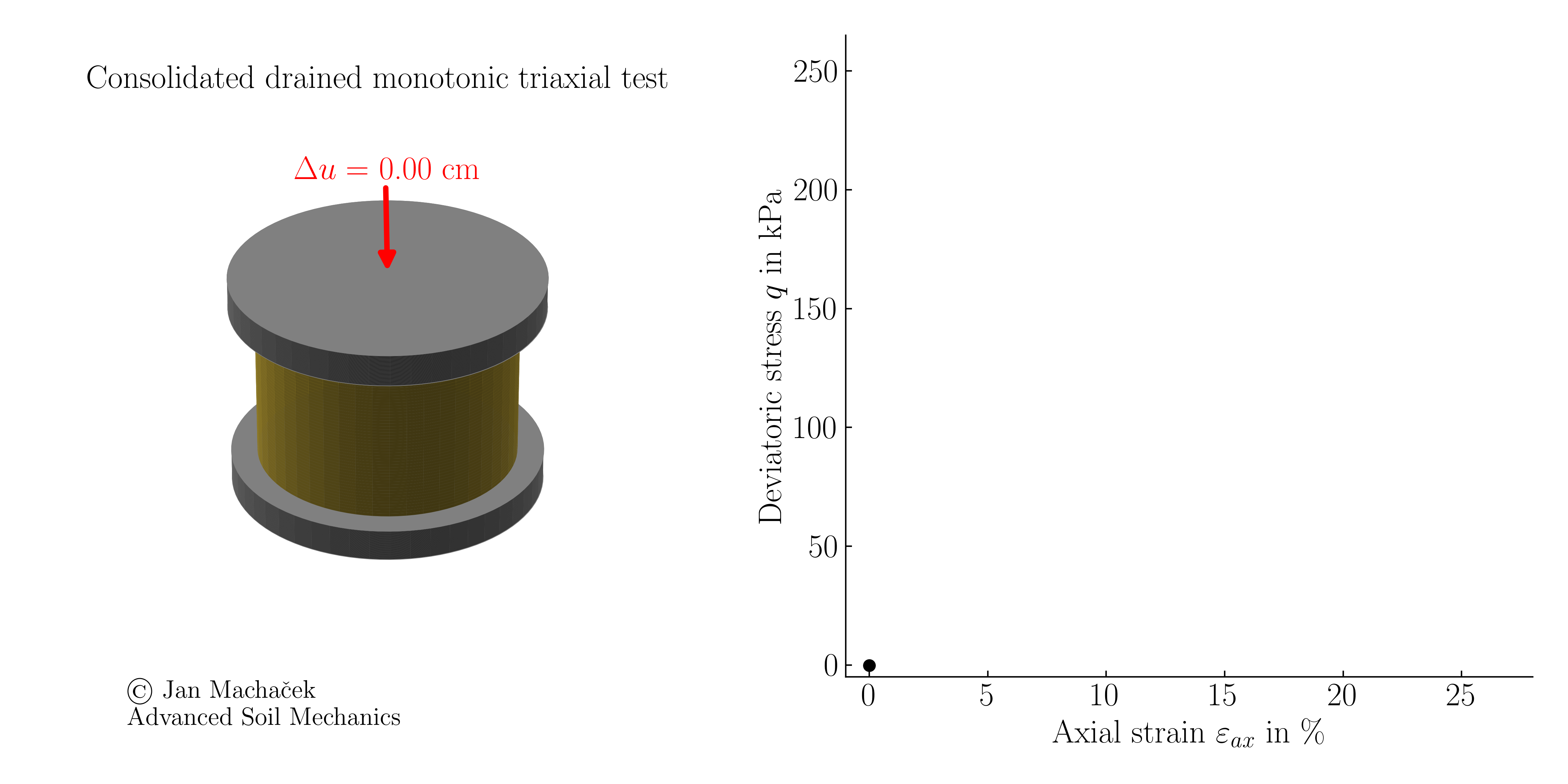Consolidated drained monotonic triaxial test (click to play)

In a triaxial test, the soil specimen (usually cylindrical) is subjected to an all-around confining pressure \(\sigma_3\) and an additional axial load. The stresses can be simplified as:

Axial Stress (Vertical Stress): \(\sigma_{ax} =\) confining pressure + additional axial stress due to applied load
Radial Stress (Horizontal Stress): \(\sigma_2 = \sigma_3 =\) confining pressure

Triaxial loading conditions further imply that:

The confining pressure is applied uniformly in all radial directions. As a result, there are no differential stresses acting tangentially on the specimen's surface, eliminating the possibility of shear strain in the radial direction.
The axial load applied to the specimen is vertical and acts along the central axis of the cylindrical specimen. Because of this, there's no lateral component of the axial load that might introduce shear.
The cylindrical shape of the specimen ensures that the state of stress at any given point within the specimen remains consistent (given that the sample is homogenous). This means that, theoretically, no rotational or tangential stresses develop within the specimen due to its shape.
The top and bottom plates of the triaxial apparatus ensure that the applied load remains axial and prevents any lateral movement or rotation of the sample. Thus no shear strains are introduced due to the boundary conditions.
The sample is isotropically confined, thus \(\sigma_2 = \sigma_3 = \sigma_r\) holds.

Given the above, the simplified stress and strain tensors for triaxial conditions in Cartesian coordinates (assuming z as the vertical axis) are:

\[ \boldsymbol{\sigma} = \begin{bmatrix} \sigma_r & 0 & 0 \\ 0 & \sigma_r & 0 \\ 0 & 0 & \sigma_{ax} \\ \end{bmatrix} ~~~\text{and}~~~ \boldsymbol{\varepsilon} \begin{bmatrix} \varepsilon_r & 0 & 0 \\ 0 & \varepsilon_r & 0 \\ 0 & 0 & \varepsilon_{ax} \\ \end{bmatrix} \]

Deviatoric strain \(\varepsilon^q\)

The understanding of stress and strain states under triaxial conditions is crucial for understanding the further content of the course. Particularly for studying soil behaviour under various loading scenarios, knowledge of the triaxial stress state is essential. For triaxial conditions, the Roscoe invariants simplify to:

\[ \begin{aligned} p &= \dfrac{1}{3} (\sigma_{ax} + 2\sigma_r) \\ q &= \sigma_{ax} - \sigma_r \end{aligned} \]

and the corresponding strain invariants:

\[ \begin{aligned} \varepsilon^{vol} &= \varepsilon_{ax} + 2\varepsilon_r \\ \varepsilon^q &= \frac{2}{3}\left(\varepsilon_{ax} - \varepsilon_r\right) \end{aligned} \]

Notice: \(q\) and \(\varepsilon^q\) are slightly modified compared to the original formulation of the invariants such that \(q\) can be either positive or negative

To understand the origin of the factor \(\frac{2}{3}\) in the definition of deviatoric stress let us recall the general definition of Roscoes second invariant:

\[ \varepsilon^q = \sqrt{ \dfrac{2}{3} \varepsilon_{ij}^\ast \varepsilon_{ij}^\ast } \]

With the deviatoric strain tensor for triaxial conditions,

\[ \varepsilon^\ast_{ij} = \begin{bmatrix} \varepsilon_{r} - \frac{1}{3} \varepsilon^{vol} & 0 & 0 \\ 0 & \varepsilon_{r} - \frac{1}{3} \varepsilon^{vol} & 0 \\ 0 & 0 & \varepsilon_{ax} - \frac{1}{3} \varepsilon^{vol} \\ \end{bmatrix} \]

the deviatoric strain \(\varepsilon^q\) is calculated as:

\[ \begin{aligned} \varepsilon^q &= \sqrt{\frac{2}{3} \left( \left(\varepsilon_{ax}- \dfrac{1}{3} \left( \varepsilon_{ax} + 2\varepsilon_r \right) \right)^2 + 2 \left(\varepsilon_r- \dfrac{1}{3} \left( \varepsilon_{ax} + 2\varepsilon_r \right) \right)^2 \right)} \\ &= \sqrt{\frac{2}{3} \left( \left(\dfrac{2}{3}\varepsilon_{ax}- \dfrac{2}{3} \varepsilon_r \right)^2 + 2 \left(- \dfrac{1}{3} \varepsilon_{ax} + \dfrac{1}{3}\varepsilon_r \right)^2 \right)} \end{aligned} \]

which can be simplified to:

\[ \begin{aligned} \varepsilon^q &= \frac{2}{3}\sqrt{\left(\varepsilon_{ax} - \varepsilon_r\right)^2}\\ &= \frac{2}{3} \left| \varepsilon_{ax} - \varepsilon_r \right| \end{aligned} \]

In order to distinguish between compression and extension above equation is modified such that the deviatoric stress can be positive (compression) or negative (extension) yields the well known equation for the deviatoric strain:

\[ \varepsilon^q = \frac{2}{3} \left(\varepsilon_{ax} - \varepsilon_r\right) \]

A. Lees, Geotechnical finite element analysis: a practical guide. 2016. ↩