Basics of Soil Dynamics – soil behaviour under dynamic loading / at (very) small strains

Soil Dynamics - a brief (!) introduction...

Soil dynamics is an extensive subject area whose comprehensive introduction contains enough content for a separate lecture "Soil Dynamics". Unfortunately, this cannot be achieved within the scope of this lecture. The following chapter is therefore merely an introduction to the topic and is intended to raise awareness of various important aspects.

In the previous section we focused on the formation of earthquakes, their role in soil liquefaction and the assessment of the latter. We learned that earthquakes have their origin mainly from tangential or transform plate movements, characterized by lateral shearing of tectonic plates. The movement of these plates is not a continuous process; rather, it is often impeded by the mechanical interlocking of plate boundaries. This leads to a gradual accumulation of shear stress along the fault lines. When the accumulated shear stress surpasses the fault's capacity to withstand it, a sudden displacement occurs, releasing the stored energy as seismic waves. These seismic events generate various types of waves, including surface waves, compressional (P-) waves, and shear (S-) waves.

This section introduces

• how different wave types propagate through soil,
• different causes for the emission of seismic waves
• Geometrical and Material damping
• the dynamic interaction between foundations and soil,
• laboratory tests to measure „dynamic“ soil properties (stiffness and damping) and
• empirical relations for „dynamic“ soil properties

Propagation of waves through soil

The dynamic excitation of the ground leads to the propagation of different types of waves in the soil. Let us first introduce the terminology of direction of propagation and direction of polarisation:

• Direction of propagation refers to the path along which a wave travels through a medium. In the context of soil, this would be the trajectory that the wavefront takes as it moves through the soil layers.

• Polarization, in wave mechanics, describes the orientation of the oscillations in the medium relative to the direction of wave travel. For mechanical waves in solids, polarization can dictate whether the particles in the medium move back and forth in a longitudinal wave or move perpendicularly to the direction of wave travel in a transverse wave.

Compressional wave

The first type of waves is the Compressional wave, or P-wave (P for primary). In the case of P-waves, the polarization direction coincides with the propagation direction. This means that particles - or soil grains, in the case of granular soils - oscillate parallel to the wave's travel direction. The following animation depicts this behavior:

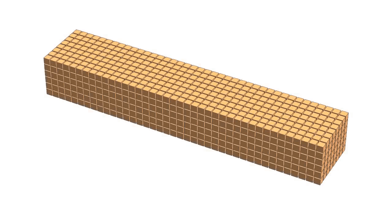Figure 1. Particle movement and direction of wave propagation of compression waves.¹ (click to play)

The propagation speed of P-waves can be derived from theory of isotropic elasticity as

\[ c_P = \sqrt{\dfrac{M}{\rho}} \]

with the soils constrained modulus \(M\) and the soil density \(\rho\). The propagation of this type of wave involves volume changes, i.e. during wave propagation some zones of the soil are compressed while some others experience dilatancy. In above animation zones that are compressed are shortened in the direction of propagation while zones that dilate are lengthened in the direction of propagation.

Linear isotropic elasticity

Earlier discussions, such as those in the chapter on Critical State Soil Mechanics highlight that soil stiffness is in general not accurately modeled by linear elasticity. Nevertheless, the strains induced in soil by wave propagation are typically minimal, which validates the application of elasticity theory in this context.

For an isotropic linear elastic material with Young's modulus \(E\) and Poisson's ratio \(\nu\) the bulk modulus \(K\), the shear modulus \(G\) and the constrained modulus \(M\) are defined as follows:

\[ \begin{aligned} K &= \dfrac{E}{3(1-2\nu)} \\ G &= \dfrac{E}{2(1+\nu)} \\ M &= K + \dfrac{4}{3}G \end{aligned} \]

Shear waves

The second type of wave is the shear wave, also termed transversal or S-wave (S for secondary). Shear waves are characterized by the absence of volume changes during propagation; they involve only shear deformations. The particles move perpendicular to the direction of wave propagation—that is, the polarization is orthogonal to the propagation direction. According to the theory of isotropic elasticity, the velocity of shear wave propagation, \(c_s\), is given by:

\[ c_S = \sqrt{\dfrac{G}{\rho}} \]

Here, \(G\) represents the soil's shear modulus, and \(\rho\) is the soil density. Since the shear modulus \(G\) is typically much lower than the constrained modulus \(M\), the velocity of S-waves is generally lower than that of P-waves.

Figure 2. Particle movement and direction of wave propagation of shear waves.¹ (click to play)

Rayleigh waves

The Rayleigh (or R) wave, unlike the P and S waves, is a surface wave that arises from the boundary condition of zero stress at the ground surface. Rayleigh waves are confined to the vicinity of the ground surface, propagating primarily in the region between the ground surface and a depth equal to the wavelength of the Rayleigh wave, denoted as \(\lambda_R = \frac{c_R}{f}\). At the depth of \(\lambda_R\), the amplitude of the Rayleigh wave is only 20% of the amplitude at the ground surface, indicating a rapid decline with depth.

As a Rayleigh wave propagates, soil particles move along an elliptical path in a counter-clockwise direction, exhibiting a greater amplitude of displacement in the vertical direction than in the horizontal direction (illustrated in the animation below).

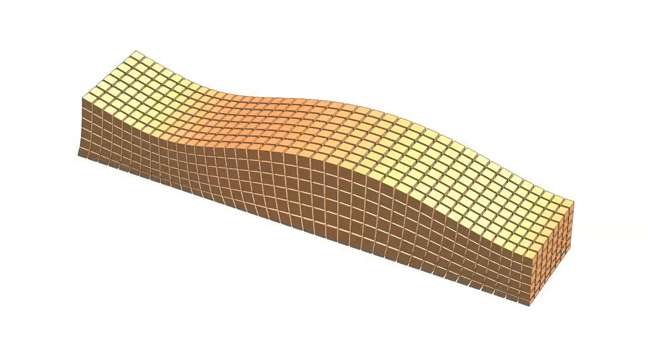Figure 3. Particle movement and direction of wave propagation of Rayleigh waves.¹ (click to play)

The velocity of R waves is slightly slower than that of S waves. The propagation speed of Rayleigh waves can be estimated using the equation:

\[ c_R \approx c_S \dfrac{0.862+1.14\nu}{1+\nu} \]

where \(c_S\) is the shear wave velocity and \(\nu\) is Poisson's ratio.

Chronology of deformations at the ground surface

The propagation velocities of all three types of waves, as a function of Poisson's ratio \(\nu\), are depicted in the figure below. The shear wave velocity is used as the baseline, meaning all wave velocities are divided by \(c_S\). Consequently, the curve for the S wave velocity is constant at 1 in this diagram, regardless of \(\nu\). The P wave is the swiftest, with the greatest propagation speed. The velocity differential between P and S waves grows with increasing Poisson's ratio. At \(\nu = 0.5\), representing an incompressible soil, the P wave velocity theoretically tends toward infinity, although this is a physical impossibility in practical scenarios. The Rayleigh wave moves at a pace slightly less than the S wave, with this disparity being more notable at smaller values of \(\nu\) and diminishing as \(\nu\) approaches 0.5.

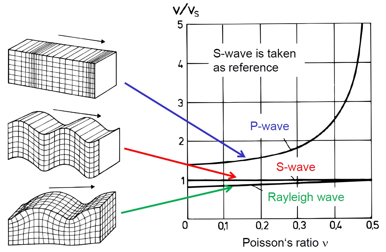
Figure 4. Comparison of P, S, and R wave velocities in dependence on Poisson's ratio. The shear wave velocity is taken as reference.

Recording horizontal and vertical deformations at the ground surface during the propagation of these waves from a distant source, such as an earthquake's epicenter, reveals that the P wave arrives first, followed by the S wave, and finally the R wave. The R wave's amplitude exceeds that of the P and S waves, largely due to energetic factors and differences in geometrical damping - a concept that entails the reduction of wave amplitude with distance due to the spreading of wave energy over a larger area. These aspects are further elaborated upon in the following subsection. Due to their significant amplitudes, R waves are often the main culprits of structural damage during earthquakes. S waves, on the other hand, have the potential to cause soil liquefaction, an effect detailed in the concluding chapter.

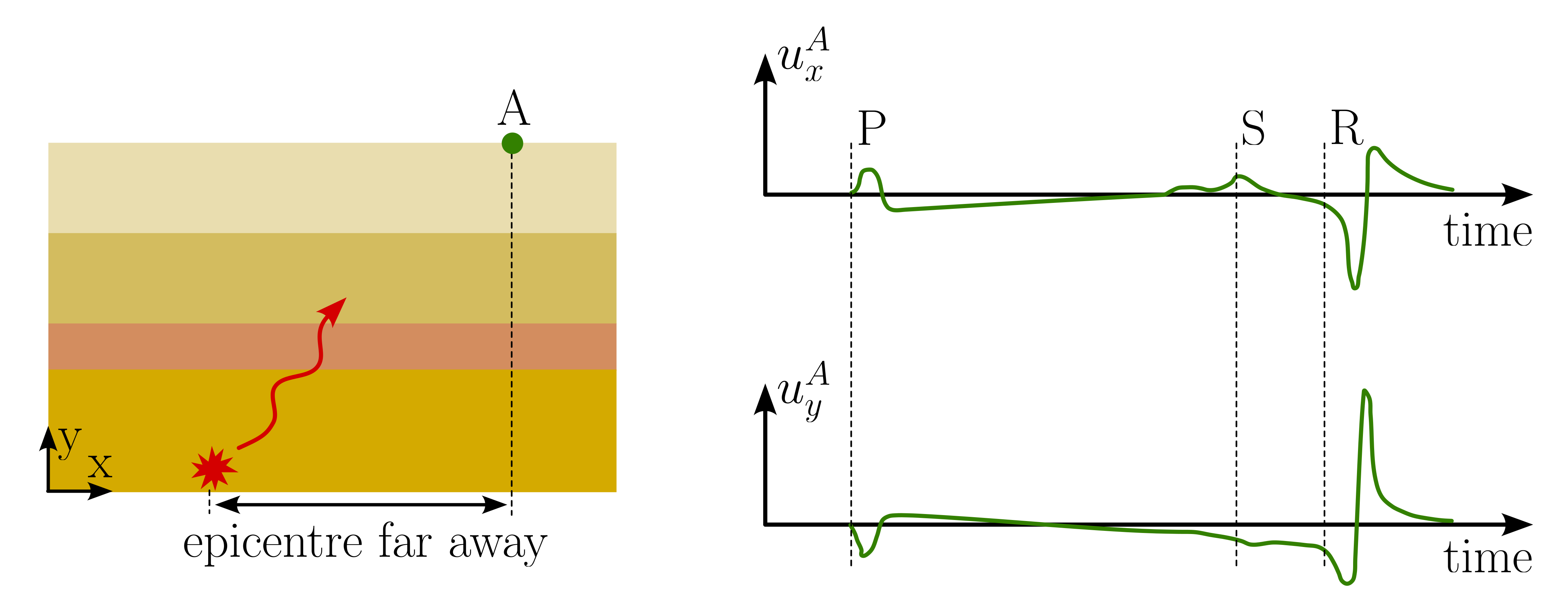
Figure 5. Ground surface displacements induced by seismic waves from an earthquake (with the epicenter far from the observation point).

Emission of waves

"Internal" source

Wave sources can be located in the ground. These typically include earthquakes or vibrations from underground transport routes in tunnels or during pile driving from a certain penetration depth of the pile. The resulting waves propagate as P and S body waves; surface waves occur only when they reach the surface.

An important aspect here is the wave propagation in the direction of the ground surface. Typically, a layered subsoil is present, the individual layers of which can vary greatly in soil type (and therefore stiffness). Even within a homogeneous soil layer of sufficient thickness, stiffness generally increases with depth due to the increase in confining pressure.

This is important because wave propagation in a layered medium with variable stiffness (and density) is fundamentally different from wave propagation in a homogeneous material. At each interface between materials of different dynamic properties, incident wave energy is split into reflected and transmitted components, as depicted in Case A of Figure 6.

Figure 6. Reflected and refracted waves resulting from incident (A,B) P-wave, (C) SV-wave, and (D) SH-wave. (SH: direction og motion is anitplane and perpendicular to the cross section of the subsoil, SV: soil particles move inside the plane)

The amount of wave energy that is transmitted or reflected depends on the impedance ratio \(\alpha_z\), defined for a single interface as:

\[ \alpha_z = \dfrac{\rho_1 v_1}{\rho_2 v_2} \]

Here, \(\rho\) represents the density, and \(v\) the wave propagation velocity of the materials on each side of the interface. Contrary to the perpendicular approach of the P-wave in Case A, waves generally encounter interfaces at oblique angles. When the angle of incidence deviates from 90° and the velocities on either side of the interface differ (\(v_1 \neq v_2\)), transmitted waves are refracted, leading to a change in wave direction and to the formation of "new" wave types. This is illustrated for different incident waves in Cases B - D of above figure.

The angle of refraction is uniquely related to the angle of incidence by the ratio of the wave velocities of the materials on each side of the interface. Snell's law indicates that waves will be refracted towards the normal when moving from higher- to lower-velocity materials. Consequently, waves ascending through horizontal layers of decreasing velocity will refract increasingly towards the vertical, as shown in Figure 7.

Figure 7. Refraction of an S-wave through series of successively softer layers (lower \(E, v\)). Reflected rays are not shown.

"External" source

Waves can also emitted by external sources on the ground surface such as by foundations when subjected to dynamic loading, as depicted in the example below.

Figure 8. Waves emitted by a foundation subjected to dynamic loading, modified from ².

In such cases, in the near field, predominantly within about one wavelength \(\lambda_R\) from the source, body waves (P and S waves) primarily dictate the propagation characteristics. Beyond this range, in the far field, surface wave propagation (R waves) becomes the dominant mode on the surface.

Magnitude of \(\lambda_R\)

Assuming a typical shear wave velocity of \(c_S\approx 200\) m/s and a Poisson ratio of \(\nu \approx 0.25\), the propagation velocity of the Rayleigh wave can be estimated:

\[ c_R \approx c_S \dfrac{0.862+1.14\nu}{1+\nu} = 200 \dfrac{0.862+1.14 \cdot 0.25}{1+0.25} = 183 ~\text{m/s} \]

The wave length \(\lambda_R = c_R/f\) for different frequencies is then

\(f\)	\(\lambda_R(c_R=183 ~\text{m/s})\)
0.1 Hz	1830 m
1 Hz	183 m
10 Hz	18.3 m
30 Hz	6.2 m

At any given moment, P waves will have propagated to a distance where the soil is compressed within a half-spherical zone (depicted in red), followed by a subsequent zone where the soil experiences dilation. Simultaneously, the leading edge of the slower S waves, closer to the foundation, shears the soil along the wavefront (indicated in yellow), resulting in alternating positive and negative shear stresses or strains.

The displacement amplitude observed at a specific distance from the foundation diminishes compared to that measured directly at the source, as demonstrated in the figure below.

Figure 9. Decrease of displacement amplitude with increasing distance to the foundation due to geometrical and material damping.

This reduction in amplitude is attributed to two types of damping: geometrical and material:

• Geometrical damping occurs because the cross-sectional area through which the waves pass expands with distance from the excitation point. For P and S waves propagating into the half-space, this area takes the shape of a growing half-spherical front. To conserve energy, the amplitude of the waves diminishes as the wave energy is distributed over a larger cross-sectional area.
• Material damping, on the other hand, is due to internal friction between soil particles. This friction arises from the relative movements of particles during wave propagation, converting some of the wave energy into heat and consequently attenuating the wave.

Geometrical Damping

In case of a point source and a harmonic excitation the P or S waves travelling in the full space show a decrease of the amplitude being proportional to the reciprocal value of the distance \(r\) to the source according to the relationship Amplitude

\[ \text{Amplitude} \sim r^{-n} ~~~\text{or}~~~ A(r) = A_0 \left( \dfrac{r}{r_0} \right)^{-n} \]

where \(A_0\) is the amplitude at measured at distance \(r_0=0\) m from the source. The amount of geometrical damping varies with the wave type and the nature and extent of the excitation source, as summarized in the table below:

Excitation Type	Source Type	Full / Half Space	Surface
		P, S wave	P, S wave	R wave
Harmonic	Point source	1.0	1.0	0.5
	Linear source	0.5	0.5	0.0
Pulsed	Point source	1.5	1.5	1.0
	Linear source	1.0	1.0	0.5

Exponents \(n\) describing geometrical damping according to the relationship Amplitude \(r^{-n}\) with the distance \(r\) to the excitation source

• For a point source under harmonic excitation, the amplitude of P or S waves in full space decreases inversely with the distance \(r\), resulting in an amplitude-distance relationship with an exponent \(n\) of 1.0.
• The same exponent applies for P and S waves travelling into the half-space, away from a point source at the ground surface.
• The amplitude of P and S waves along the surface decays more rapidly (\(n = 2.0\)), while Rayleigh waves experience less geometrical damping (\(n = 0.5\)), leading to their comparatively larger amplitudes at a distance from the source.
• For a linear source, the damping is less pronounced, with all exponents \(n\) decreased by 0.5 compared to a point source.
• Conversely, for pulsed excitation, the damping is more significant, with all exponents \(n\) increased by 0.5 relative to harmonic excitation.

In case of a point source and a harmonic excitation the P or S waves traveling in the full space show a decrease of the amplitude being proportional to the reciprocal value of the distance \(r\), i.e. the exponent \(n\) of the relationship Amplitude \(\sim r^{-n}\) is 1.0.

The same exponent applies for P and S waves traveling into the half-space, away from a point source at the ground surface. The amplitude of the P and S waves propagating along the surface of the half space declines even faster (\(n = 2.0\)), while the geometrical damping is lower for the Rayleigh waves (\(n = 0.5\)). The considerably lower geometrical damping is the reason for the larger amplitudes of the Rayleigh waves compared to P and S waves measured at the ground surface in some distance to the source of excitation. If a linear source of excitation is considered instead of a point source, then the geometrical damping is lower. Compared to the point source, all exponents n are reduced by 0.5. In case of a pulsed excitation it is the other way around: The geometrical damping is higher. Compared to the harmonic oscillation all exponents n are increased by 0.5.

Material Damping

In addition to its elastic properties, natural ground always exhibits material damping, resulting from the internal friction between soil particles. This friction arises from the relative movements of particles during wave propagation, converting some of the wave energy into heat and consequently attenuating the wave.

Therefore, in addition to the reduction due to radiation damping, the amplitudes of the waves as they propagate will also be reduced due to energy dissipation in the material (material damping).

The impact of material damping on the attenuation of wave amplitudes is integrated with the effects of geometrical damping using a multiplicative model:

\[ A(r) = A_0 \left( \dfrac{r}{r_0} \right)^{-n} e^{-\alpha_D(r-r_0)} \]

The amplitude decay coefficient \(\alpha_D\) is depending on the damping ratio \(D\) and the wave length \(\lambda\). The following relation holds:

\[ \alpha_D \approx 2 \pi \dfrac{D}{\lambda} \]

This formula implies that material damping has a proportionally greater effect on longer waves, given the same damping ratio.

In the near field of a vibration source, material damping has little effect compared to the reduction in amplitude due to propagation. In the far field, however, it can be of critical importance, especially for surface waves. This is shown in below figure.

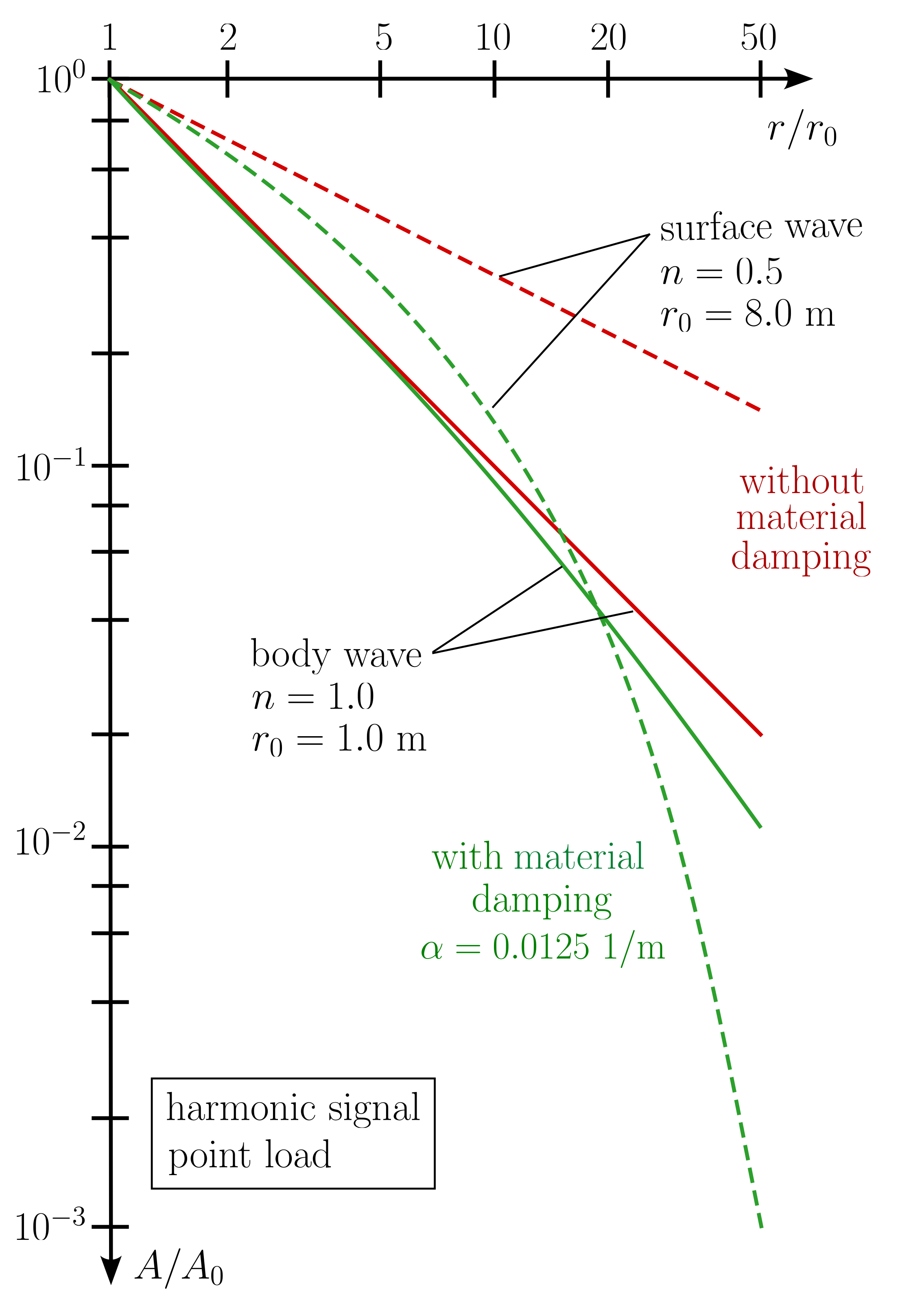
Figure 10. Influence of material damping on the amplitude decay of body waves and surface waves. Homogeneous soil as well as equal frequency and wave length are assumed. Modified from ²

"Dynamic" soil properties

A dynamic loading usually means a cyclic (repeated) loading of the soil, i.e. the strain and stress components oscillate in time during the dynamic action. One can distinguish

• a dynamic loading as a cyclic loading of the soil where inertia effects are of relevance
• a quasi-static cyclic loading where the cycles are applied rather slowly, so that inertia effects are negligible.

Under dynamic loading, soils typically experience small strains, generally less than \(10^{-3}\). This level of strain is considerably lower compared to what is often induced by monotonic loading. An exception to this occurs during soil liquefaction in an earthquake, where effective stresses temporarily vanish, leading to significantly larger strains (see Earthquakes and assessment of liquefaction). In the following (sub)sections we will concentrate on the

• Shear modulus \(G\)
• Damping ratio \(D\)
• Poisson's ratio \(\nu\)

of soils at small strains as these are needed for the calculation of wave propagation as described in above sections.

Given that small strains are predominant in most soil dynamics problems, it is usual to consider soil as exhibiting non-linear (but) elastic behavior. This non-linearity stems from the shear stress-shear strain relationship's inherent non-linear characteristics. The figure below qualitatively demonstrates this relationship, as observed in a simple shear test. For a monotonically increasing initial load, the soil's base stiffness diminishes progressively between load points. This change in stiffness can be quantified either by the tangent modulus (the tangent at the load point) or by the secant modulus (the secant between the origin and the load point). The maximum shear modulus at the start of loading, denoted as \(G_{max}\), represents the peak stiffness for small deformations under a monotonic initial load. When the strain amplitude exceeds this point (\(\gamma \approx 10^{-5}\)), the material response remains elastic (i.e., no plastic strains are formed), but the secant shear modulus diminishes. Plastic strains, along with a continuing reduction in the secant shear modulus, emerge once the strain surpasses a specific threshold (\(\gamma \approx 10^{-4}\)). A typical relationship for \(G-\gamma\) is illustrated on the right-hand side of Figure 11.

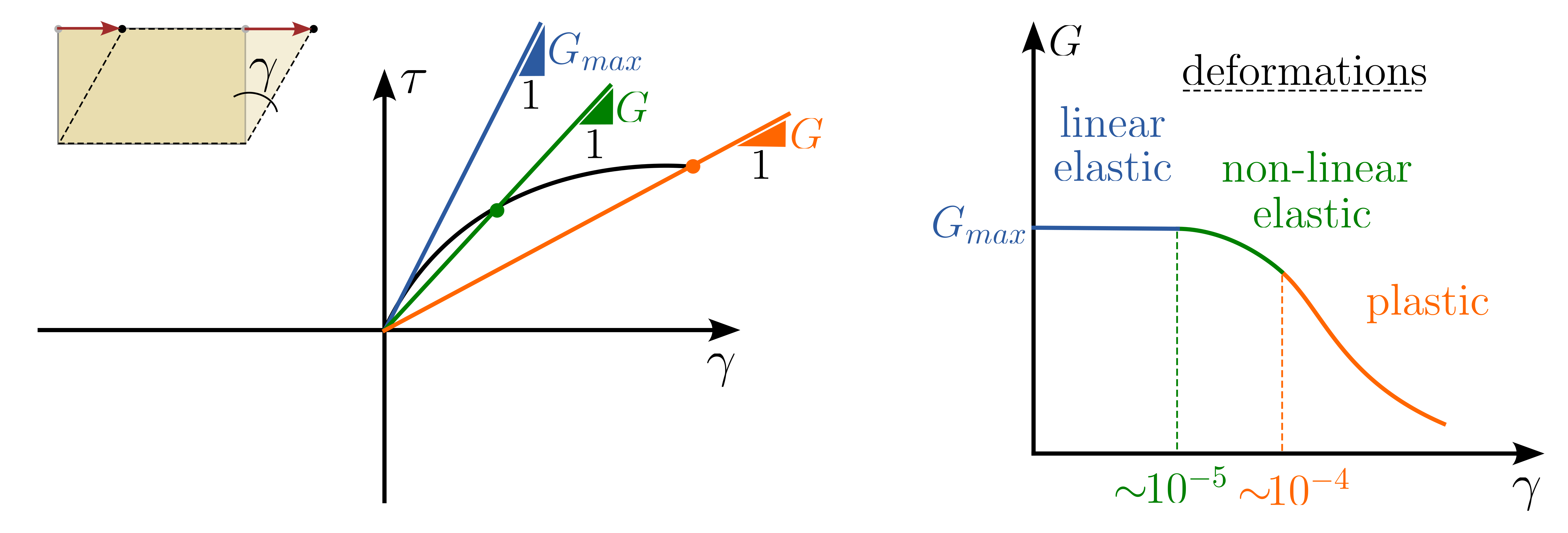
Figure 11. Qualitative soil behaviour under monotonic primary loading

The \(G-\gamma\) relationship illustrated in Figure 11 is also applicable to soils under cyclic loading. When cycles with minimal strain amplitudes \(\gamma^{ampl}\) are applied, the stress-strain relationship \(\gamma-\tau\) follows a linear path without hysteresis, inclined at an angle corresponding to \(G_{max}\). This linear behavior is depicted in Figure 12 as the blue stress-strain path. As the shear strain amplitude increases, the stress-strain relationship begins to form an area, depicted in green in Figure 12.

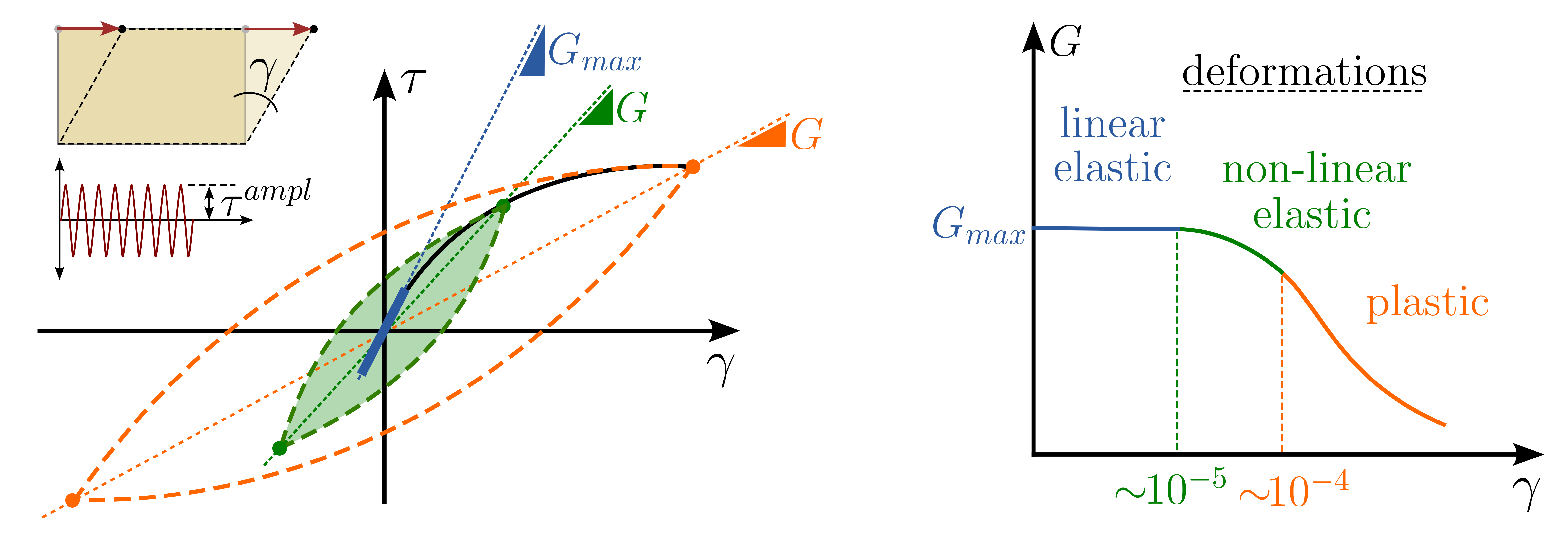
Figure 12. Qualitative soil behaviour under cyclic loading with different strain amplitudes.

Drawing a line through the maximum points of the \(\gamma-\tau\) hysteresis loop reveals its inclination is equal to the secant shear modulus \(G\) and smaller than \(G_{max}\). Further increase in strain amplitude, represented by the orange area, results in an expanded loop area and a corresponding decrease in the average inclination of the loop, indicating a reduction in the secant shear modulus. The expansion of the loop area with each \(\gamma-\tau\) cycle is indicative of material damping – the larger the area, the greater the material damping effect.

The material damping results from the ratio of the dissipated energy during a single cycle \(\Delta W\) to the elastic storage energy \(W\) (the elastic energy at the maximum shear strain during that cycle.). For an illustration of \(W\) and \(\Delta W\) refer to Figure 13 a). The damping properties are usually provided by means of the damping capacity \(\Psi\) or the damping ratio \(D\):

\[ \Psi = \dfrac{\Delta W}{W} ~~~\text{and}~~~ D = \dfrac{\Psi}{4\pi} = \dfrac{\Delta W}{4 \pi W} \]

The amount of damping increases with increasing cyclic shear strain amplitude \(\gamma\), see Figure 14 b).

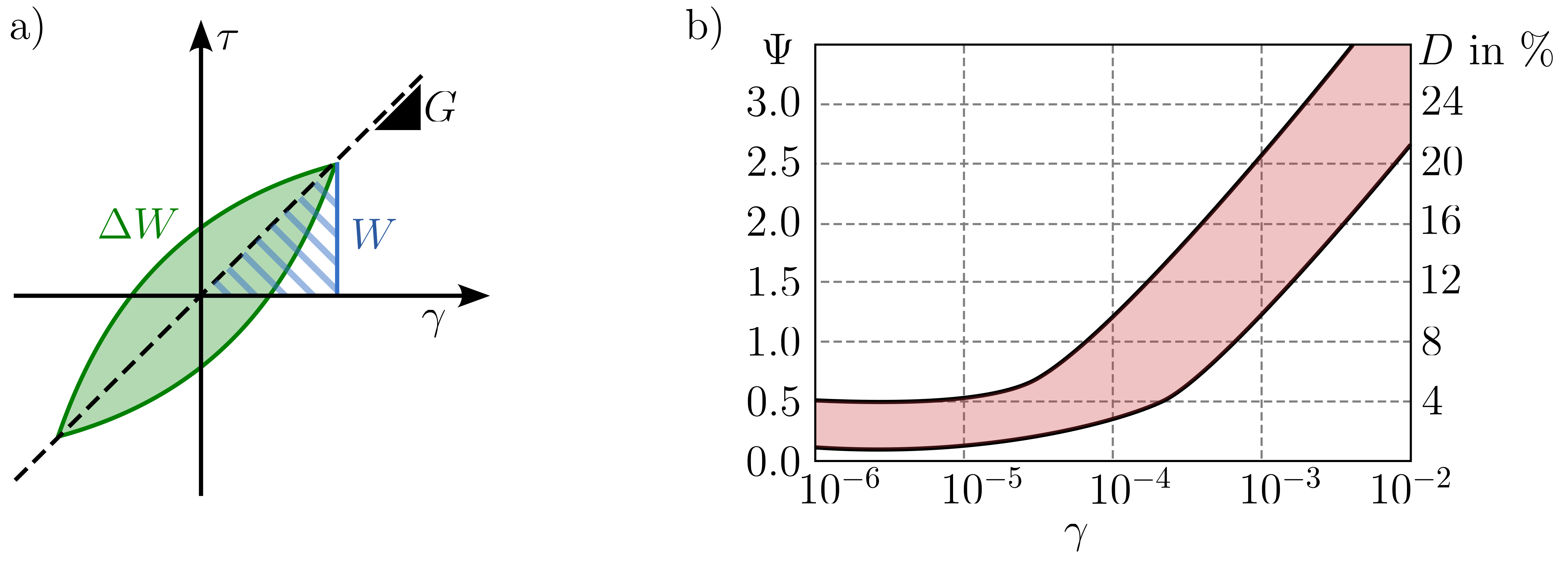
Figure 13. a) Hysteretic stress-strain curve, b) Damping capacity \(\Psi\) and damping ratio \(D\) as a function of the shear strain amplitude, modified from ².

A distinction between static and dynamic shear modulus is not physically justified. Different shear moduli can occur depending on the existing loading condition, the type of load to be applied (monotonic or cyclic) and the magnitude of the deformations that occur. A more appropriate title for this section would thus be "soil properties at small strains".

A different interpretation small/elastic and large/plastic deformations has been established from the evaluation of various types of cyclic tests in Vucetic (1994)³. As long as the shear strain amplitude is less than the so-called linear limit shear strain \(\gamma_{tl}\), the behaviour remains linear-elastic and no permanent deformation or development of excess pore water occurs. \(\gamma_{tl}\) is defined as a function of the plasticity index of the soil and assumes values between approx. \(5\cdot 10^{-6}\) for sands/gravels and approx. \(5\cdot10^{-5}\) for highly plastic clays. If the strain amplitude is exceeded, permanent deformations occur, the magnitude of which depends on the relative density, the degree of saturation, drainage conditions, the magnitude of the mean effective stress, the shear strain amplitude and the number of cycles. Beyond a further threshold known as the volumetric shear strain \(\gamma_{tv}\), significant permanent deformations and excess pore water pressures arise, affecting the soil's mechanical properties. According to ³, \(\gamma_{tv}\) is a function of the plasticity index, with values ranging from \(1.5\cdot10^{-4}\) for sands/gravels to approximately \(1.5\cdot10^{-3}\) for highly plastic clays (refer to Fig. 14). The original values in ³ have been supplemented by more recent results in Hsu & Vucetic (2004)⁴. Permanent soil deformations occur when strain amplitudes fall between \(\gamma_{tl}\) and \(\gamma_{tv}\).

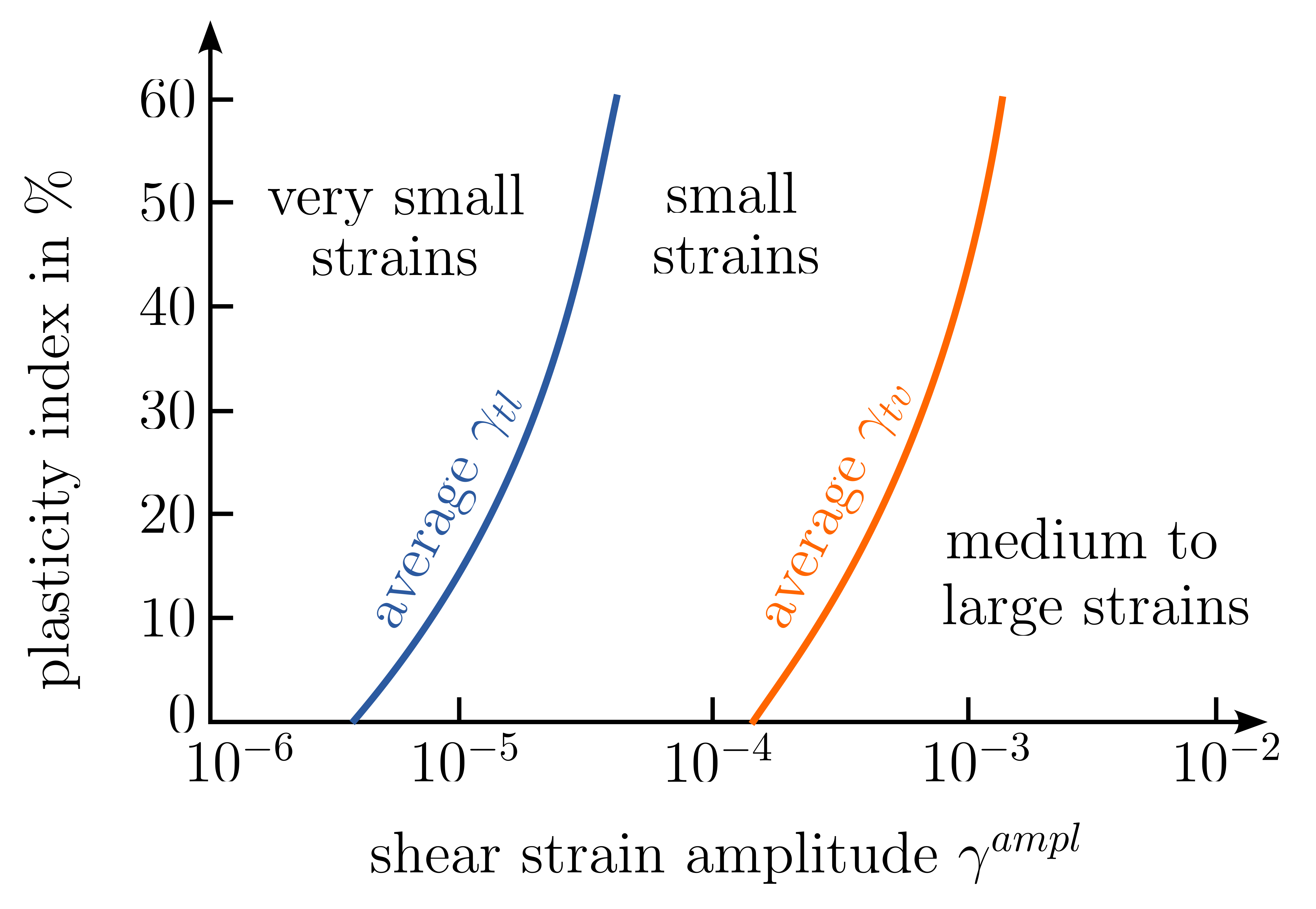
Figure 14. Limiting shear strains as a function of plasticity index, modified from ³.

The material constants necessary for the evaluation of the wave velocities or the design of a foundation subjected to dynamic loading - shear modulus \(G(\gamma)\), the Poisson's ratio \(\nu\) and the damping ratio \(D\) - can be determined using different methods:

• Field testing
• Laboratory tests performed on undisturbed or disturbed samples
• Empirical formulas and equations or diagrams correlating the SPT or CPT sounding resistance with the dynamic shear modulus

Rough estimates of \(G_{max}\)

Mean values for \(G_{max}\) are given in the table below. A major disadvantage of all tables is the wide range of values and the lack of information on how and under what conditions they were determined, i.e no information is provided about corresponding stress state or density are provided. Therefore, values outside the limits given in the table may well occur. However, the values are certainly useful as a first estimate of the order of magnitude.

Non-cohesive soils²Cohesive soils²Rock²

Soil Type	\(G_{max}\)
Loose sand	50 MPa - 120 MPa
Medium dense sand	70 MPa - 170 MPa
Dense sandy gravel	100 MPa - 300 MPa

Soil Type	\(G_{max}\)
Mud, clay	3 MPa - 10 MPa
Loam, soft to stiff	20 MPa - 50 MPa
Clay, semi-solid to hard	80 MPa - 300 MPa

Rock Type	\(G_{max}\)
Layered, brittle	1 GPa - 5 GPa
Solid	4 GPa - 20 GPa

Rough estimates for \(\nu\)

Generally, the static Poisson's ratios are used for which reference values² are given below

• Sand and Gravel: \(0.25 \leq \nu \leq 0.35\)
• Silt, depending on sand and clay content: \(0.35 \leq \nu \leq 0.45\)
• Clay, depending on water content: \(0.45 \leq \nu \leq 0.49\)

Empirical formulas based on laboratory tests

For small projects or feasibility studies when field or laboratory test data are not available yet, \(G_{max}\) can be estimated from simple empirical formulas, based on the void ratio and the pressure acting in the soil. Several authors have proposed empirical relationships for \(G_{max}\), mostly from results of resonant column experiments. A more general formula is given in ⁵:

\[ G_{max} = S ~F(e) \left( \dfrac{p_0^\prime}{p_{atm}}\right)^n p_{atm} \]

where \(S\) is a factor depending on the soil type, \(F(e)\) is a function of the void ratio \(e\), \(p_0^\prime\) is the initial mean effective stress, \(n<1\) is the barotropy factor (controlling the influence of the mean effective stress) and \(p_{atm}\) is the atmospheric pressure. Resonant column tests have repeatedly shown that \(n = 0.5\) is a very good approximation for sands. Similar values of \(n\) have been found for a large number of soils. Different equations have been proposed for \(F(e)\), which demonstrates the variability of soils. With regard to over-consolidation ratio OCR, it was found that an increase in OCR, and therefore in consolidation stress, leads to an increase in \(G_{max}\), which is greater for plastic clays than for sands. The effect of OCR is sometimes considered by incorporating a factor OCR\(^k\) in the equation for \(G_{max}\):

\[ G_{max} = S ~F(e) \left( \dfrac{p_0^\prime}{p_{atm}}\right)^n p_{atm} ~OCR^k ~~~\text{with:}~~~ k = \dfrac{PI}{\sqrt{1+3PI^2}} \]

The exponent \(k\) depends on the plasticity index \(PI\) (given in decimals). In ² and ⁵ it is recommended to estimate \(G_{max}\) for most practical applications in the context of pre-dimensioning, with sufficient accuracy for clays and sands using \(S=625\), \(n=0.5\) and \(F(e)=1/(0.3+0.7e^2)\), i.e.

\[ G_{max} = 625 \dfrac{1}{0.3+0.7e^2} \left( \dfrac{p_0^\prime}{p_{atm}}\right)^{0.5} p_{atm} ~OCR^k \]

The atmospheric pressure can be assumed to \(p_{atm}\approx 100\) kPa. To get a better feel for the influence of the different factors on the calculated shear modulus, the above equation is analysed for different void ratios \(e\) and plasticity indices \(PI\) and plotted in Figure 15.

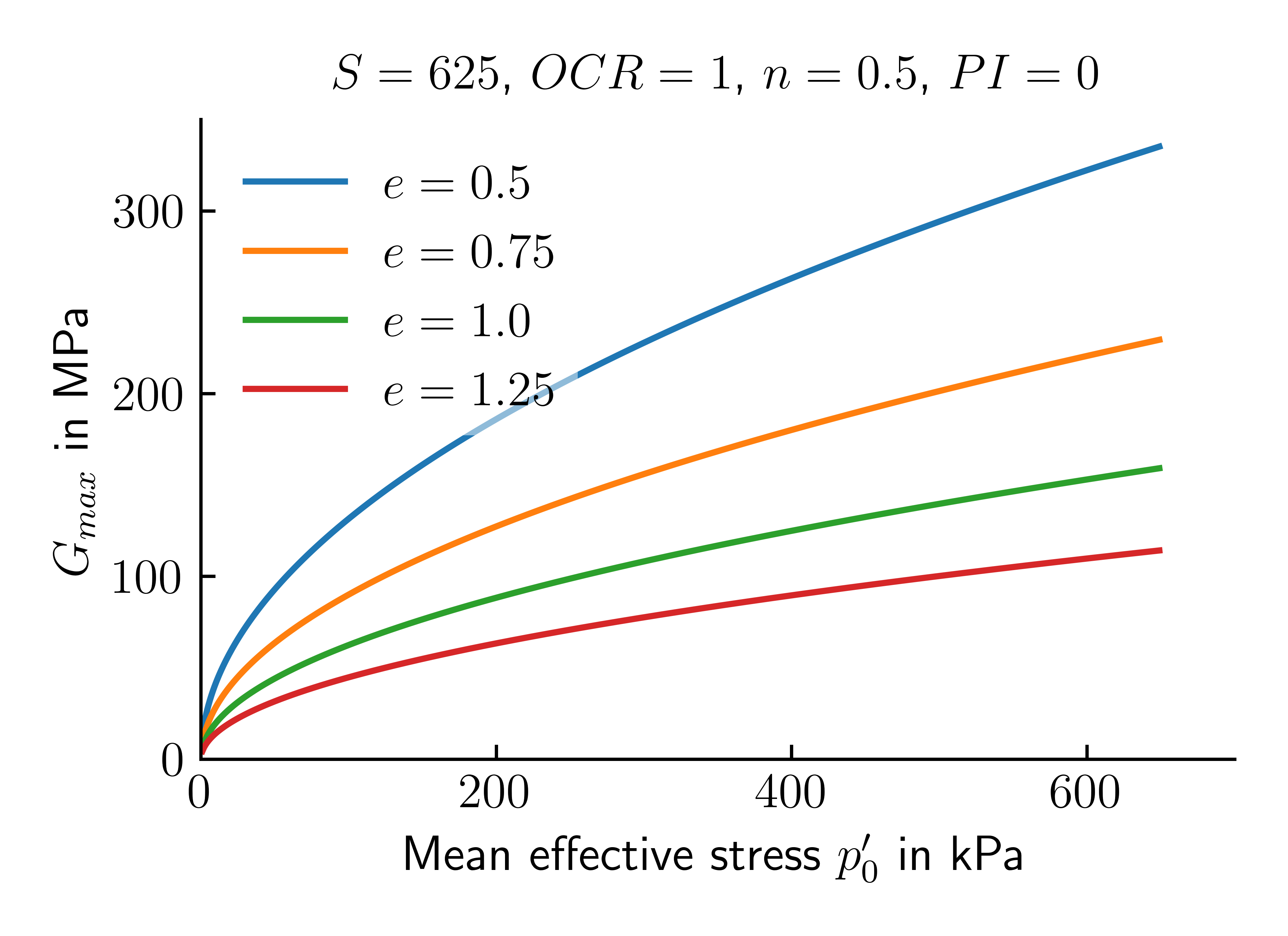
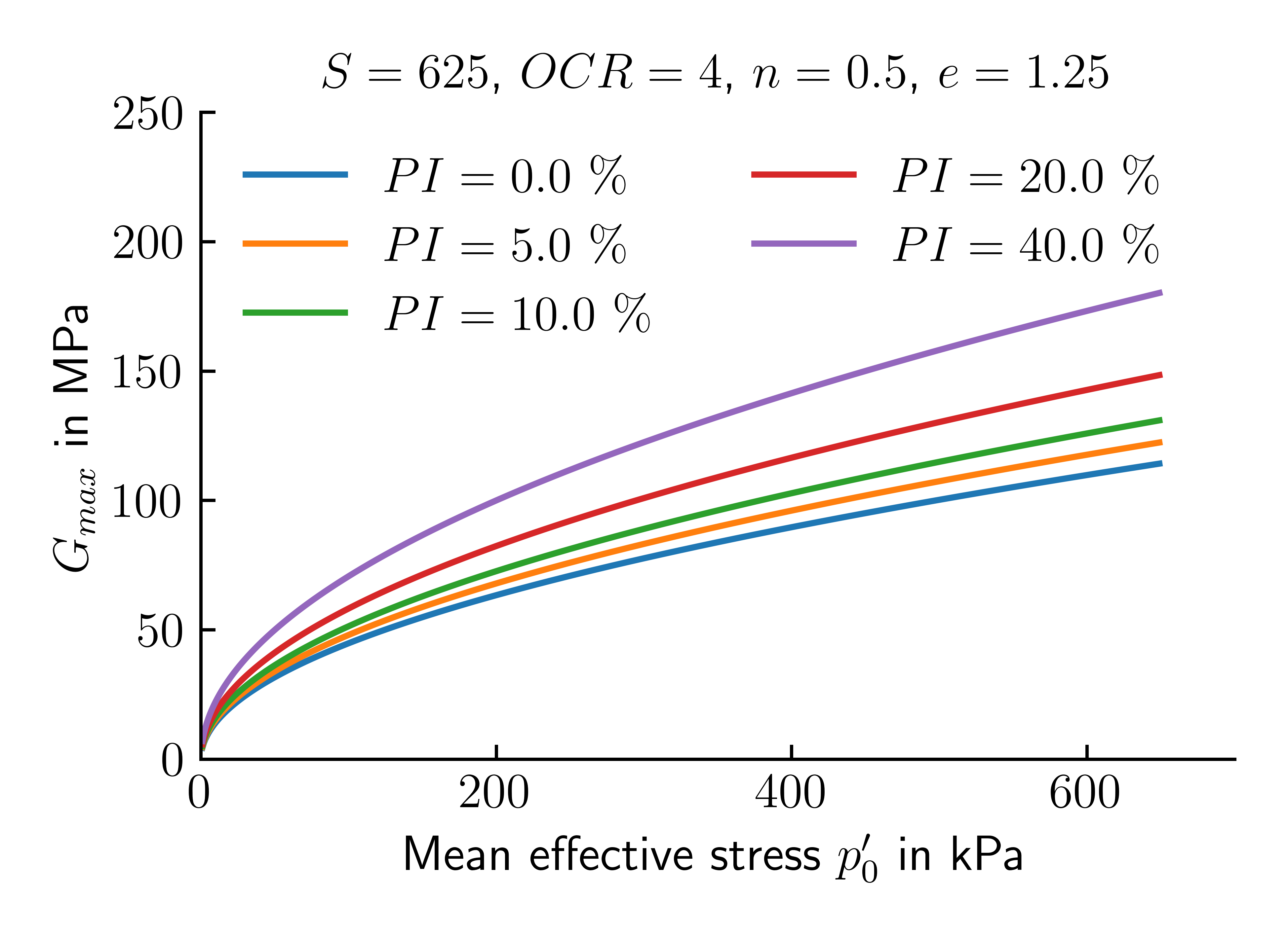
Figure 15. \(G_{max}\) according to the empirical formula as a function of mean effective stress \(p^\prime_0\) for given void ratios \(e\), over-consolidation ratio OCR and plasticity indices \(PI\).

Compared to the rough estimates given in above tables, the range on values fits reasonably well.

It is important to emphasise that it is in the nature of empirical equations that they are only a rough estimate and not a substitute for field or laboratory studies. Their range of validity is limited to the range of data on which they are based - an important aspect that is too often ignored. A more elaborate summary of different correlations is provided in ⁵ to which reference is made.

Numerous empirical formulas can be found in the literature describing the decrease of the shear modulus \(G\) or the ratio \(G/G_{max}\) with increasing strain amplitude \(\gamma_{ampl}\) as displayed in Figures 10 and 11. In ² and ⁵ the following relation is provided for \(\gamma_{ampl} < 1 \%\):

\[ \dfrac{G}{G_{max}} = \min \left\{ \dfrac{1.03}{1+\dfrac{19 \gamma_{ampl}^{0.8}}{1+(PI/10)^{1.3}}}; 1 \right\} \]

Note that in above equation, the shear strain amplitude \(\gamma_{ampl}\) and the plasticity index \(PI\) have to be given in %. The equation as to be bound by the maximum value of one since for very small strains values of \(G/G_{max} > 1\) are calculated. Non-cohesive soils, such as sands, correspond to the limit case \(PI=0\). The influence of the plasticity index and the shear strain amplitude on the ratio \(G/G_{max}\) is demonstrated in Figure 16.

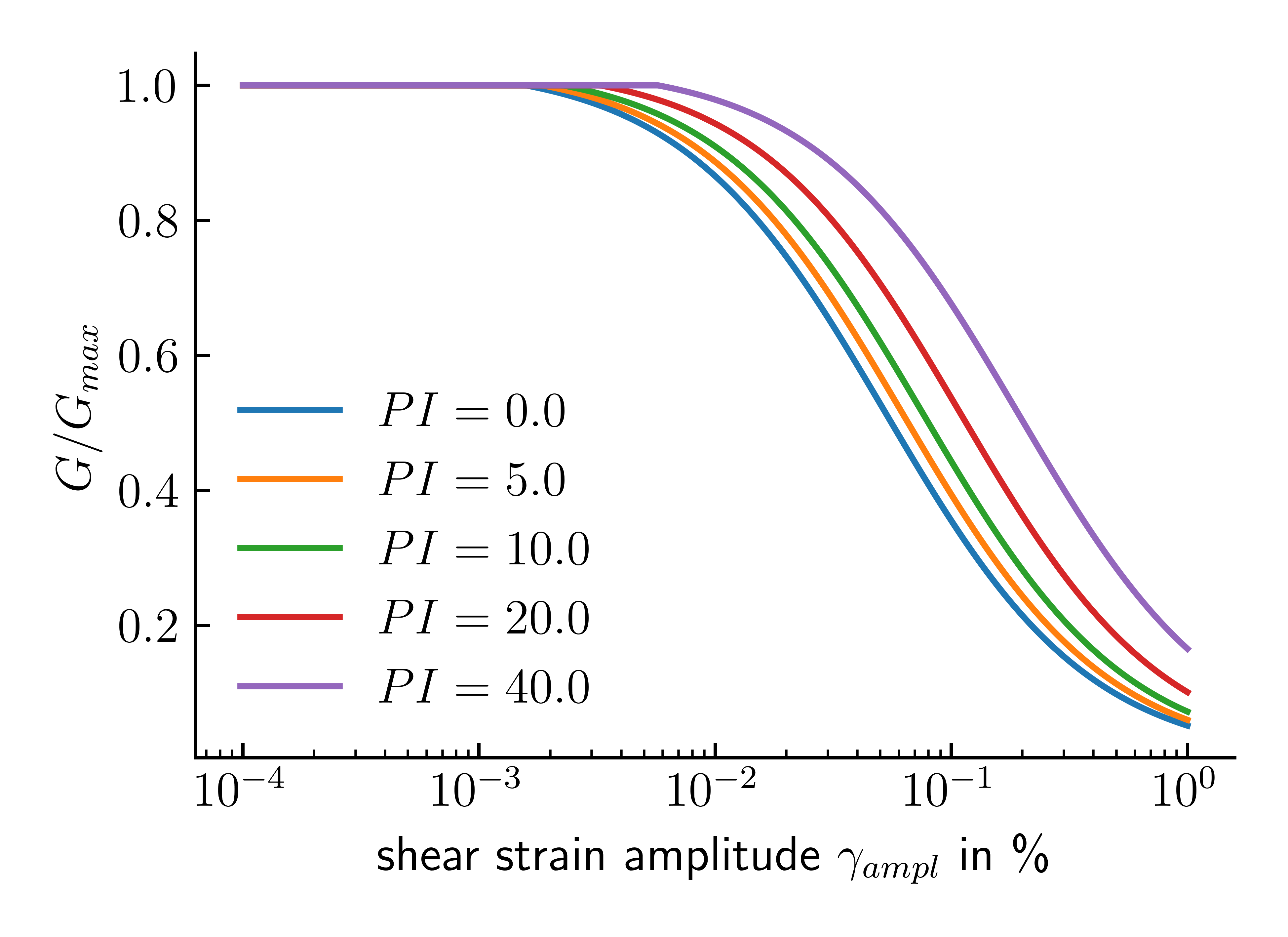
Figure 16. Estimated ratio \(G/G_{max}\) for different shear strain amplitudes and plasticity indices.

From Figure 16 (and corresponding equation) we can see that as the plasticity index \(PI\) of the soil increases, the level of cyclic shear strain needed to induce significant nonlinear stress-strain response and stiffness degradation also increases.

A corresponding relation for the Damping ratio \(D\) is given by

\[ D = 2 + \dfrac{24.5 - 0.2 PI}{1 + \dfrac{1}{\left(7.4 - 0.1 PI \right)\gamma^{0.8}}} \]

The influence of the plasticity index and the shear strain amplitude on the Damping ratio \(D\) is illustrated in Figure 17.

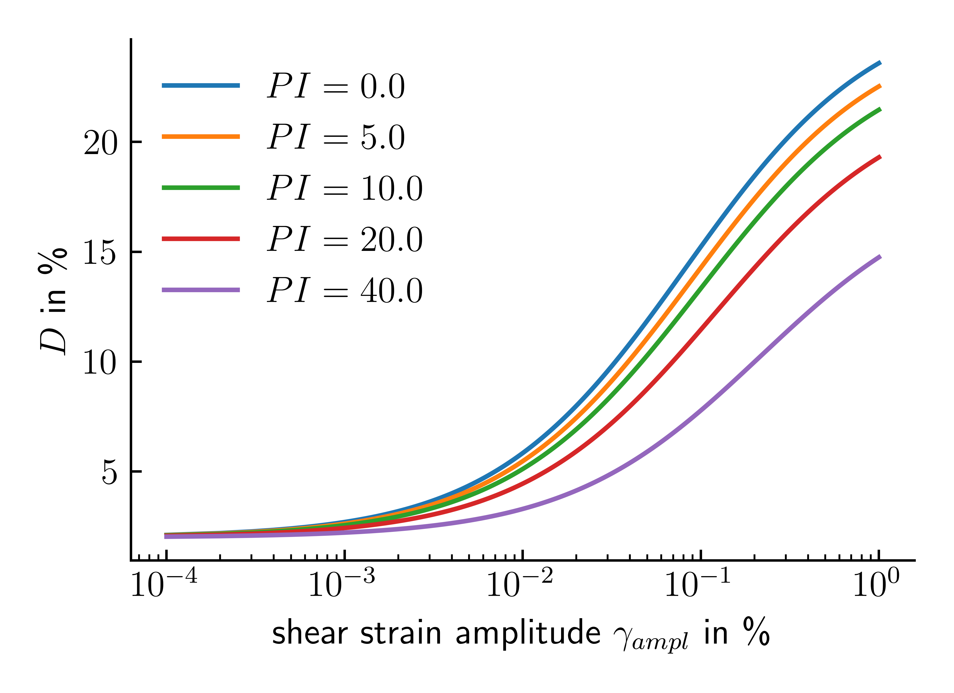
Figure 17. Estimated Damping ratio \(D\) for different shear strain amplitudes and plasticity indices.

Field and laboratory tests

Field tests have the advantage that dynamic soil parameters can be determined on a relatively large scale in undisturbed subsoil. The disadvantage, however, is that the influence of stress state and dynamic strain amplitude on the parameters obtained is usually not known. In addition, field tests only give information on soil behaviour at very small strain amplitudes in the range of \(10^{-6} \leq \gamma \leq 10^{-4}\). In laboratory tests, the dependence of the dynamic soil parameters on these variables can be determined more precisely. However, a disadvantage is the random sampling of the subsoil. Moreover, the soil material is disturbed by taking the samples and placing them in the test apparatus. While the resulting effects on gravel and sand are usually minimal if the density present in the subsoil is reproduced in the laboratory, in the case of clay this can lead to considerable differences between the results of field and laboratory tests. Experience has shown that laboratory tests generally give lower values of dynamic shear modulus than field tests.

A reliable determination of dynamic soil properties should include both field and laboratory tests.

Field tests

The majority of dynamic field tests in geotechnical engineering involve seismic measurements. These tests typically assess wave propagation in the subsoil or at the ground surface. A fundamental aspect of these measurements is recording the 'time of flight' of a seismic wave between two points. The wave velocity is calculated by using the distance between these points and the time the wave takes to travel this distance. This can also involve analyzing the wave's time of flight curve. In geophysical field tests, the compressional wave velocity (\(c_p\)) of the soil is commonly determined. However, by selecting appropriate pulse excitation and transducers, it's also possible to measure the travel time of a shear pulse and calculate the shear wave velocity (\(c_s\)) from this data.

Measuring the shear wave velocity is particularly advantageous as it allows for the direct determination of the dynamic shear modulus without relying on the Poisson's ratio \(\nu\). Below the groundwater table, accurate information can only be gleaned from measuring the compressional wave velocity if this velocity exceeds that in the water (average of approximately 1440 m/s) within the soil's grain structure. If not, the determination of shear wave velocity becomes essential.

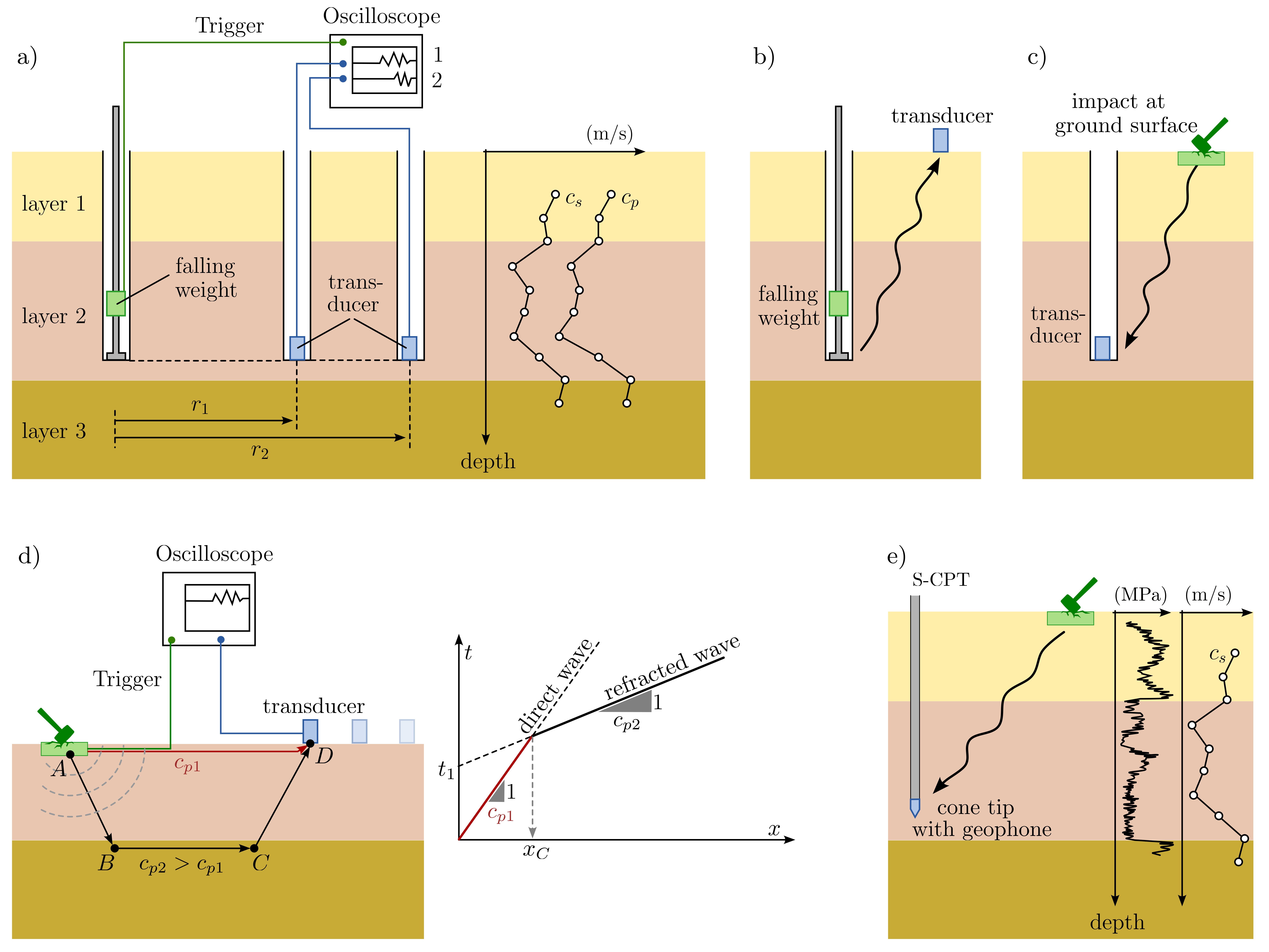
Figure 18. Summary of field tests: a) Cross-hole test, b) up-hole test, c) down-hole test, d) refraction measurement and e) seismic cone penetration test (S-CPT).

• Cross-Hole Test: As illustrated in Figure 18 a), this test involves generating and detecting seismic pulses within boreholes. These pulses can be generated and detected at the same or different depths, or even at the bottom of the boreholes. Utilizing more than two boreholes enhances the accuracy and reliability of the results. The wave paths in this test can be horizontal, inclined, straight, or curved, leading to a detailed profile of wave velocities over depth. Although cross-hole tests offer high reliability and precise results, they require significant technical and potentially financial resources.

• Single Borehole Methods: These include the down-hole and up-hole tests.

  • Down-Hole Test: Shown in Figure 18 c), this test involves generating seismic waves at the ground surface (commonly with a hammer) and detecting them at the bottom of a borehole. The measured velocities correspond to an inclined path from the source to the transducer. When conducted at various depths, these tests yield profiles of wave velocities, though interpretation might be more challenging than in cross-hole tests due to the inclined nature of the wave paths.
  • Up-Hole Test: Operating similarly to the down-hole test, but in reverse, as depicted in Figure 18 d). Here, the impact is created at the bottom of the borehole, and the waves are detected at the surface. This method is generally less complex and more cost-effective than cross-hole testing.

• Refraction Measurement: In this method, an impulse is generated at the ground surface (e.g., by a hammer blow) and recorded by transducers placed at various distances from the impact point. Particularly useful in stratified subsoils, as shown in Figure 18 e), it allows for the determination of layer boundaries but wave velocities in deeper layers must be higher than in the upper layers. The height \(H\) of the top layer in Figure 18 e) can then be calculated by

  \[ H = \dfrac{x_c}{2} \sqrt{\dfrac{c_{p2}-c_{p1}}{c_{p2}+c_{p1}}} \]

  where \(x_c\) is the distance up to which the direct wave \(c_{p1}\) is faster than the refracted wave \(c_{p2}\). If the travel time \(t\) is plotted versus the distance \(x\) (Figure 18 e), then up to the distance \(x_c\) the direct wave is faster than the refracted one. Therefore, in that range a linear curve (marked in red in the figure) is obtained being inclined by the reciprocal value of the P wave velocity \(c_{p1}\) of the upper layer. At all distances exceeding \(x_c\) the refracted wave arrives earlier than the direct one. Beyond the distance \(x_c\) the relationship between travel time and distance is governed by the refracted wave. In that range, one again obtains a linear curve, but now with the inclination being identical to the reciprocal value of the P wave velocity \(c_{p2}\) of the second layer.

• Seismic Cone Penetration Tests (S-CPT): Gaining popularity in recent years, S-CPTs, illustrated in Figure 18 e), operate on similar principles as down-hole tests. These tests integrate a receiver in the tip of a CPT probe, with excitation applied at the ground surface. As the probe penetrates the soil, wave velocities are measured at various depths. This measurement method has a clear cost advantage as no boreholes need to be drilled. In addition to the seismic velocities for the P- and S- waves, the S-CPT method typically records conventional CPT test data such as cone tip resistance, shaft friction and pore water pressure as functions of depth. This large number of information at a site is very useful to summarise and improve the interpretation of the measured values for site identification.

Poisson's ratio \(\nu\)

If dynamic field and laboratory tests are available, the Poisson's coefficient \(\nu\) can be calculated from the wave velocities of the compression wave \(c_p\) (m/s) and shear wave \(c_s\) (m/s):

\[ \nu = \dfrac{c_p^2-2c_s^2}{2(c_p^2-c_s^2)} \]

---

1. Animation created with Mathematica following https://blog.wolfram.com/2011/03/18/built-to-last-understanding-earthquake-engineering/ ↩

2. Deutsche Gesellschaft für Geotechnik, Ed., Empfehlungen des Arbeitskreises ‘Baugrunddynamik’, 2. Auflage. Berlin: Wilhelm Ernst & Sohn, 2019. ↩↩↩↩↩↩

3. M. Vucetic, ‘Cyclic Threshold Shear Strains in Soils’, J. Geotech. Engrg., vol. 120, no. 12, pp. 2208–2228, Dec. 1994, doi: 10.1061/(ASCE)0733-9410(1994)120:12(2208). ↩↩↩

4. C.-C. Hsu and M. Vucetic, ‘Volumetric Threshold Shear Strain for Cyclic Settlement’, J. Geotech. Geoenviron. Eng., vol. 130, no. 1, pp. 58–70, Jan. 2004, doi: 10.1061/(ASCE)1090-0241(2004)130:1(58). ↩

5. K. J. Witt, Ed., Grundbau-Taschenbuch Teil 1: Geotechnische Grundlagen, 8. Auflage. Berlin: Ernst, Wilhelm & Sohn, 2017. ↩↩↩↩

6. B. O. Hardin and V. P. Drnevich, ‘Shear Modulus and Damping in Soils: Design Equations and Curves’, J. Soil Mech. and Found. Div., vol. 98, no. 7, pp. 667–692, Jul. 1972, doi: 10.1061/JSFEAQ.0001760. ↩