Mohr-Coulomb

The Mohr-Coulomb model is a widely, if not the most, used constitutive model in geotechnical practice. Strictly speaking, the name Mohr-Coulomb for the material model is not correct, as the name merely refers to the model used to describe the limit state in the stress space. The formulation of the model corresponds to a Linear Elastic Perfectly Plastic (LEPP) modelling approach. This means that the material behaves linearly elastic until the limit state is reached, i.e. $\sigma = \sigma_f$ (see Figure 1). When the limit state is reached (and only then!) a further increase in stress is not possible and irreversible (plastic) deformations occur.

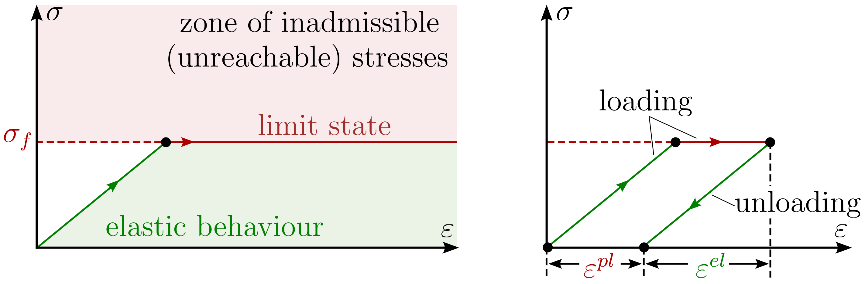
Figure 1. Illustration of a Linear Elastic Perfectly Plastic (LEPP) material behaviour.

The LEPP Mohr-Coulomb model has three main components:

Decomposition of the total strain into an elastic (reversible) and a plastic (irreversible) portion:

\[ \varepsilon_{ij} = \varepsilon_{ij}^{el} + \varepsilon_{ij}^{pl} \]

A schematic of this decomposition of strain is shown on the right.hand-side of Figure 1. Stresses developing due to changes in elastic strain $\varepsilon_{ij}^{el}$ are calculated assuming an isotropic linear elastic material behaviour. This part of the model is not discussed further in this section and reference is made to Section Isotropic linear elasticity.
The decomposition of strain into an elastic and a plastic portion implies the existence of a limit state separating admissible from inadmissible stress states. The mathematical equation that describes this separation is called the yield surface.

Yield surface

The LEPP Mohr-Coulomb constitutive model uses the well-known Mohr-Coulomb (MC) criterion as yield surface dividing the stress space into an admissible and an inadmissible region. From the bachelors courses we are familiar with the representation of the MC failure criterion in $\tau-\sigma_n^\prime$ space, where $\tau$ is the shear stress and $\sigma_n^\prime$ is the (effective) normal stress. In Section Triaxial test of this lecture we learned a different representation of the MC failure criterion in $p-q$ space, where $p$ adn $q$ are the Roscoe stress invariants. For the sake of completeness both representations are illustrated in Figure 2.

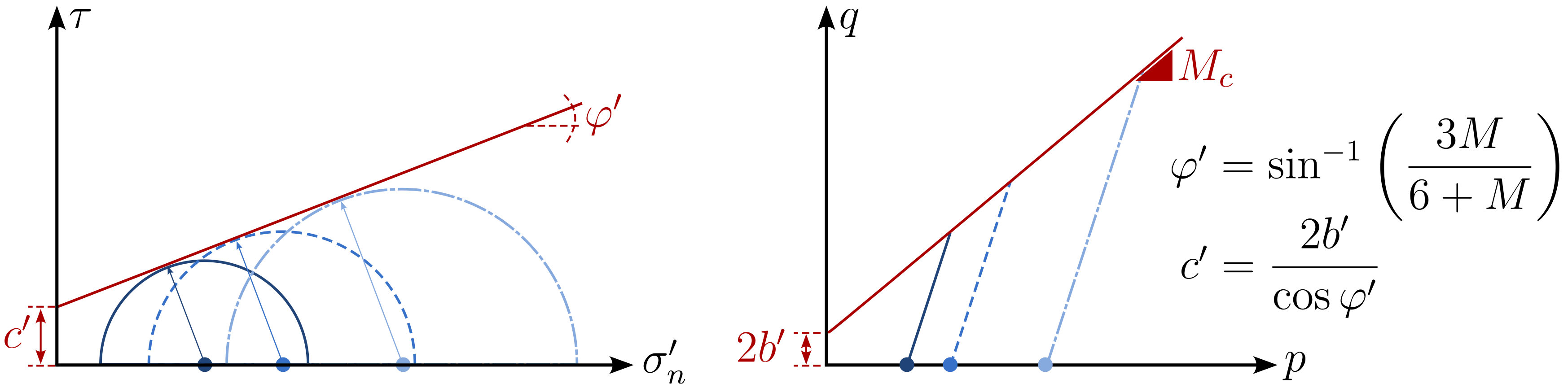
Figure 2. Mohr Coulomb failure line (red) in $\tau-\sigma_n^\prime$ (left) and $p-q$ space (right).

Figure 2 only shows the MC failure criterion for triaxial compression. However, already in Section Undrained monotonic triaxial extension tests on sand we learned that stress paths deviating from triaxial compression can result in a different maximum shear stress in the failure state. This becomes obvious looking at the results of a series of true triaxial tests presented by Lade¹ depicted in Figure 3. It can be seen, that "triaxial compression" and "triaxial extension" are only two special cases, and many other stress states (grey dots) exist.

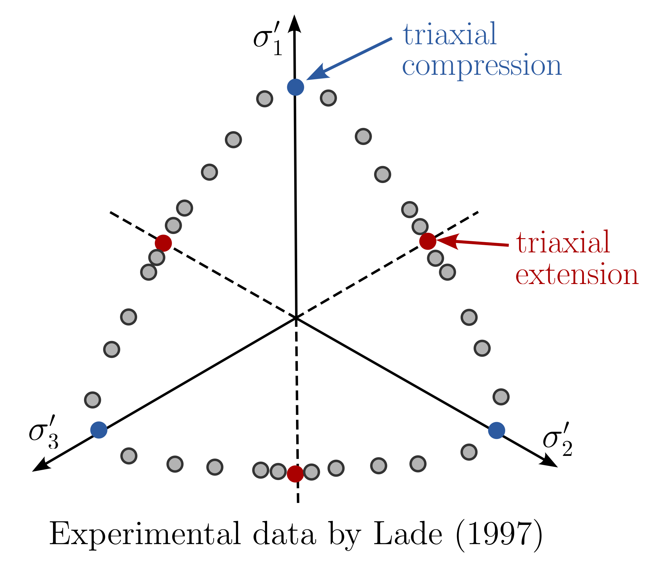
Figure 3. Shape of the limit state in principal stress space based on experimental data from Lade (1997).

For general stress states, the MC failure criterion has a hexagonal shape in principal stress space as depicted in Figure 4 for a non-cohesive soil ($c^\prime=0$).

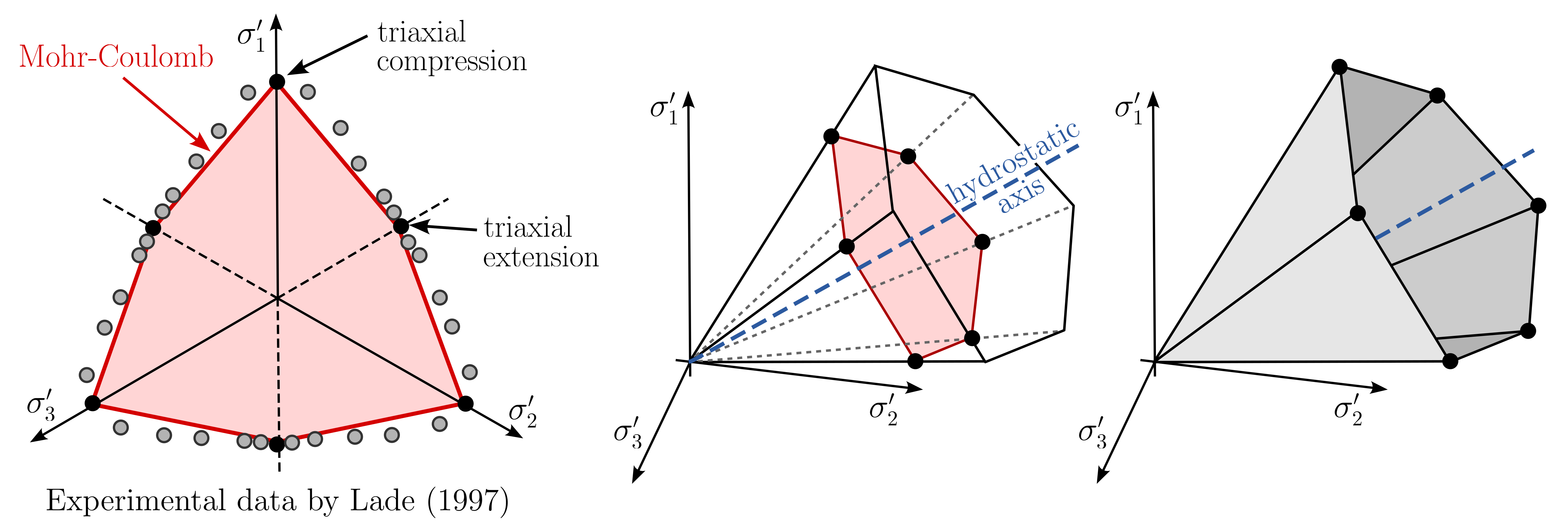
Figure 4. Mohr-Coulomb failure surface in principal stress space for the case of zero cohesion ($c^\prime=0$).

As can be seen from Figure 4, the full Mohr-Coulomb failure condition is composed of six individual conditions when formulated in terms of principal stresses. Failure occurs if one of below conditions is violated:

\[ \begin{aligned} \frac{1}{2} (\sigma'_{3} - \sigma'_{1}) &\leq c' \cos \varphi' - \frac{1}{2} (\sigma'_{3} + \sigma'_{1}) \sin \varphi' \\ \frac{1}{2} (\sigma'_{2} - \sigma'_{3}) &\leq c' \cos \varphi' - \frac{1}{2} (\sigma'_{2} + \sigma'_{3}) \sin \varphi' \\ \frac{1}{2} (\sigma'_{3} - \sigma'_{1}) &\leq c' \cos \varphi' - \frac{1}{2} (\sigma'_{3} + \sigma'_{1}) \sin \varphi' \\ \frac{1}{2} (\sigma'_{1} - \sigma'_{3}) &\leq c' \cos \varphi' - \frac{1}{2} (\sigma'_{1} + \sigma'_{3}) \sin \varphi' \\ \frac{1}{2} (\sigma'_{2} - \sigma'_{1}) &\leq c' \cos \varphi' - \frac{1}{2} (\sigma'_{2} + \sigma'_{1}) \sin \varphi' \\ \frac{1}{2} (\sigma'_{1} - \sigma'_{2}) &\leq c' \cos \varphi' - \frac{1}{2} (\sigma'_{1} + \sigma'_{2}) \sin \varphi' \end{aligned} \]

For the formulation of constitutive models it is more convenient to reformulate the failure conditions into functions $f(\sigma_1,\sigma_2,\sigma_3,\varphi',c')$ that

are $>0$ if the failure condition is violated,
are $=0$ (exactly) at failure and
are $<0$ for admissible stress states

These functions are called yield functions. The 6 MC failure criteria result in 6 yield functions:

\[ \begin{aligned} f_{1a} &= \frac{1}{2} (\sigma'_{2} - \sigma'_{3}) + \frac{1}{2} (\sigma'_{2} + \sigma'_{3})\sin \varphi' - c' \cos \varphi' \leq 0 \\ f_{1b} &= \frac{1}{2} (\sigma'_{3} - \sigma'_{1}) + \frac{1}{2} (\sigma'_{3} + \sigma'_{1})\sin \varphi' - c' \cos \varphi' \leq 0 \\ f_{2a} &= \frac{1}{2} (\sigma'_{3} - \sigma'_{1}) + \frac{1}{2} (\sigma'_{3} + \sigma'_{1})\sin \varphi' - c' \cos \varphi' \leq 0 \\ f_{2b} &= \frac{1}{2} (\sigma'_{1} - \sigma'_{3}) + \frac{1}{2} (\sigma'_{1} + \sigma'_{3})\sin \varphi' - c' \cos \varphi' \leq 0 \\ f_{3a} &= \frac{1}{2} (\sigma'_{1} - \sigma'_{2}) + \frac{1}{2} (\sigma'_{1} + \sigma'_{2})\sin \varphi' - c' \cos \varphi' \leq 0 \\ f_{3b} &= \frac{1}{2} (\sigma'_{2} - \sigma'_{1}) + \frac{1}{2} (\sigma'_{2} + \sigma'_{1})\sin \varphi' - c' \cos \varphi' \leq 0 \end{aligned} \]

It can be seen from above equations, that all six functions require the same two parameters: the friction angle $\varphi^\prime$ and the cohesion $c^\prime$.

A note on the yield surface

Since the yield functions of the LEPP MC model are formulated in terms of the current stress state ($\sigma_1', \sigma_2'$ and $\sigma_3'$) and two constants ($\varphi'$ and $c'$) they are fixed in (principal stress) space. They can neither expand, shrink or rotate. Although this may seem obvious and of little importance at this point, it is a crucial feature of the LEPP MC model that distinguishes it from more advanced constitutive models, as will be seen in the following section.

Flow rule

The yield functions presented in the previous section allow a separation between admissible and inadmissible stress states. Within the admissible range, i.e. for $f_i < 0$, the material behaviour is assumed to be linearly elastic, i.e. the deformations are fully reversible. However, for stresses outside the admissible range ($f_i > 0$), a projection must be made back to the yield surface so that $f_i=0$ holds, i.e. the limit criterion is exactly satisfied. However, the price of this projection is the development of (large) plastic deformations. However, it is unclear in which direction these plastic deformations occur. This requires another mathematical model, called the flow rule: the rule governing the direction of flow,i.e. the plastic deformation. In general the flow rule is a tensorial function, similar to stress and strain.

A distinction is often made between associated and non-associated flow rules, see Figure 5. With the associated flow rule, the direction of the flow rule is perpendicular to the flow surface, i.e. parallel to its normal vector $\boldsymbol{n}$. For non-associated flow rules, the direction of the flow rule differs from that of the normal vector.

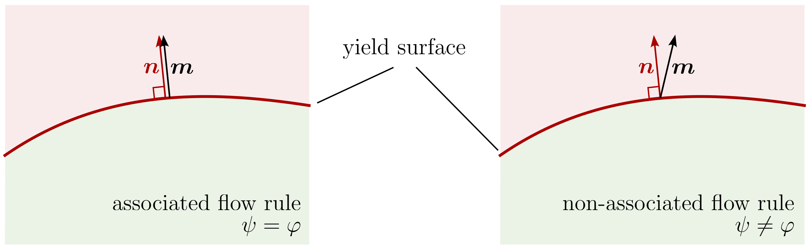
Figure 5. Left: associated flow rule $\boldsymbol{m}$ ($\psi = \varphi$), right: non-associated flow rule ($\psi \neq \varphi$). $\boldsymbol{n}$ denotes the normal vector of the yield surface.

Usually an equation for the flow rule $\boldsymbol{m}$ is not postulated directly, but introduced by formulating a suitable plastic potential $g$, whereby the following applies:

\[ \boldsymbol{m} = \dfrac{\partial g}{\partial \boldsymbol{\sigma}} \]

For the case of an associated flow rule, where $\boldsymbol{m}=\boldsymbol{n}$ applies, $g=f$ and thus $\partial g / \partial \boldsymbol{\sigma} = \partial f / \partial \boldsymbol{\sigma}$ holds. Most formulations of the LEPP MC model allow for both, an associated and a non-associated flow rule. This is realized by choosing the plastic potential $g$ similar to the flow rule $f$ but replacing the friction angle $\varphi'$ with the "dilatation angle" $\psi$:

\[ \begin{aligned} g_{1a} &= \frac{1}{2} (\sigma'_{1} - \sigma'_{2}) + \frac{1}{2} (\sigma'_{3} + \sigma'_{2}) \sin \psi - c' \cos \psi \\ g_{1b} &= \frac{1}{2} (\sigma'_{2} - \sigma'_{3}) + \frac{1}{2} (\sigma'_{2} + \sigma'_{3}) \sin \psi - c' \cos \psi \\ g_{2a} &= \frac{1}{2} (\sigma'_{1} - \sigma'_{3}) + \frac{1}{2} (\sigma'_{1} + \sigma'_{3}) \sin \psi - c' \cos \psi \\ g_{2b} &= \frac{1}{2} (\sigma'_{3} - \sigma'_{1}) + \frac{1}{2} (\sigma'_{3} + \sigma'_{1}) \sin \psi - c' \cos \psi \\ g_{3a} &= \frac{1}{2} (\sigma'_{1} - \sigma'_{2}) + \frac{1}{2} (\sigma'_{1} + \sigma'_{2}) \sin \psi - c' \cos \psi \\ g_{3b} &= \frac{1}{2} (\sigma'_{2} - \sigma'_{1}) + \frac{1}{2} (\sigma'_{2} + \sigma'_{1}) \sin \psi - c' \cos \psi \end{aligned} \]

For $\psi = \varphi'$, $g=f$ and an associated flow rule is obtained. For $\psi \neq \varphi$, $g \neq f$ a non-associated flow rule is obtained. In the LEPP MC model, dilatancy (positive plastic volumetric strain) can only be modelled with $\psi \neq \varphi$. Choosing an appropriate dilatation angle $\psi$ is the responsibility of the user.

Simulation examples

In the following some simulation examples are given demonstrating the performance of the LEPP MC model and the influence of the model parameters on the simulation results. The reference simulation assumes a granular soil with $\varphi'=30^\circ$, $c'=0$ kPa, $\psi=0^\circ$, $E=5$ MPa and $\nu=0.3$. Although arbitrarily chosen, these are representative parameters e.g. for loose sands. A drained monotonic triaxial test will be simulated starting at an initial mean effective stress of $p'_0=100$ kPa.

Figure 6. Simulation of a drained monotonic triaxial test using the LEPP Mohr-Coulomb model.

From Figure 6. the linear elastic behaviour of the LEPP MC model for stresses inside the yield surface (MC failure criterion) is obvious. Once the deviatoric stress $q$ reaches the yield surface, no further increase in $q$ or $p'$ are observed in $p'-q$ space. The simulated behavior is an elastic-perfectly plastic behavior. For $\psi=0$ the material behaviour at failure is isochoric, i.e. the plastic strain is purely deviatoric. This is well visible from the strain path in the $\varepsilon_a-\varepsilon_v$ plane of Figure 6.

Next, the effect of the dilatancy angle $\psi$ on the simulation results are demonstrated. for this we perform a parametric study. Based on the calculation just seen ($\varphi'=30^\circ$, $c'=0$ kPa, $\psi=0^\circ$, $E=5$ MPa and $\nu=0.3$), the dilatancy angle is gradually increased until $\psi=\varphi$. The results of this study demonstrating the effect of $\psi$ are summarized in Figure 7.

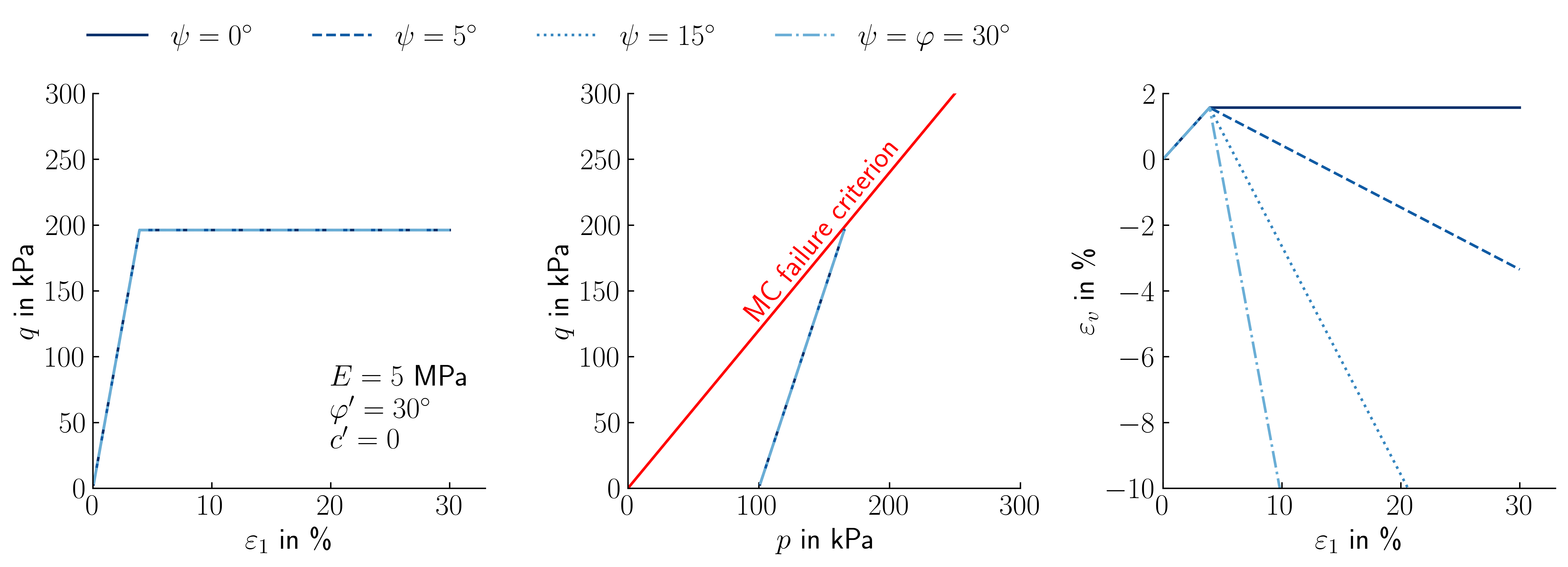
Figure 7. Influence of the dilatancy angle $\psi$ on the predicted material behaviour using the LEPP MC model for the example of a drained monotonic triaxial test.

As can be seen from Figure 7, the effect dilation in drained conditions is only visible in the variation of volumetric strain with axial strain ($\varepsilon_a-\varepsilon_v$ plane). The shear strength of the material is not affected by the choice of $\psi$. From Figure 7 it can also be seen that the increase in volume (reflected by negative $\varepsilon_v$ in the $\varepsilon_a-\varepsilon_v$ plane) grows without limits. This is clearly unrealistic, as most soils will reach a critical state at some point and further shear deformation will occur without volume changes.

In simulations facing undrained conditions, this can lead to an overestimation of shear strength. Under undrained conditions this increase in volume can not develop. As a consequence, a decrease in pore water pressure is observed. This decrease in pore water pressure increases the effective stresses which leads to a continuous increase in shear strength for shear deformations at the limit state. This effect is shown in Figure 8.

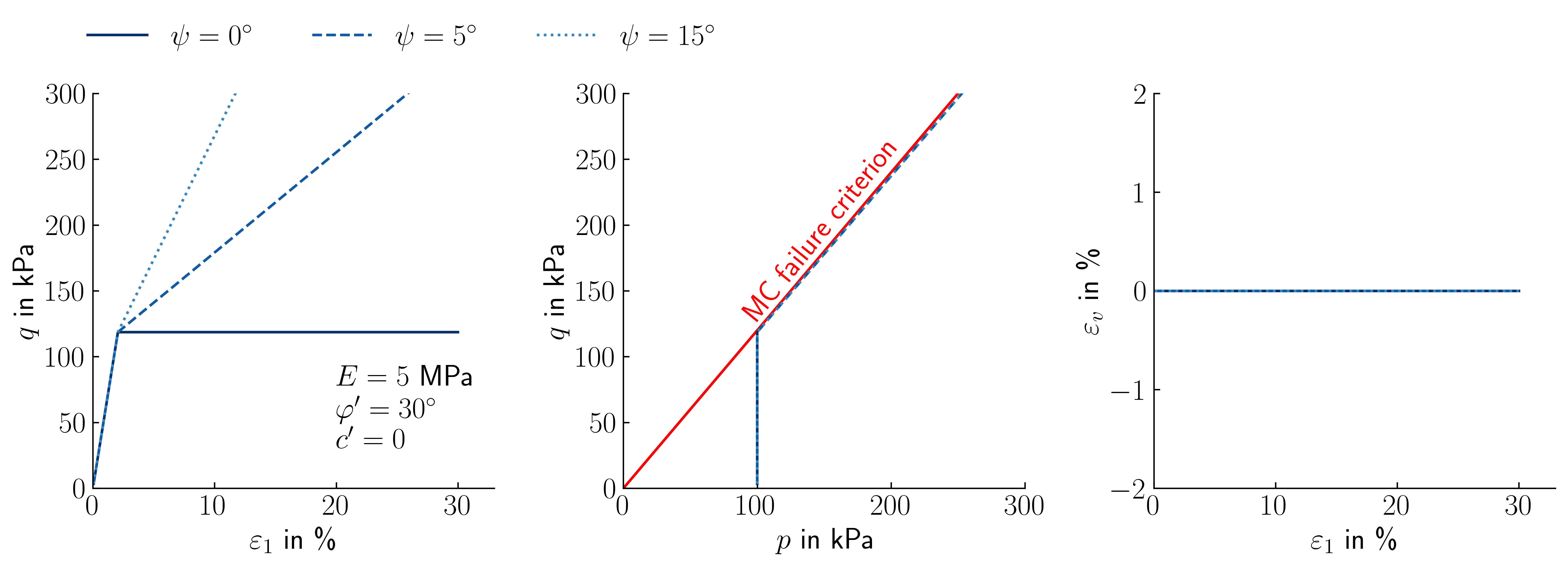
Figure 8. Influence of the dilatancy angle $\psi$ on the predicted material behaviour using the LEPP MC model for the example of an undrained monotonic triaxial test.

Parameter calibration

Elasticity

The elastic constants $E$ and $\nu$ are usually determined based on (drained) triaxial compression tests as the secant stiffness $E_{50}%$ at 50% of the maximum shear strength as explained in Section Isotropic linear elasticity.

If unloading processes, such as excavations, are to be simulated with the LEPP MC model $E_{50}$ will generally result in an overestimation of displacements. For such cases the Young's modulus should be determined as the secant stiffness during an unloading path.

Friction angle and cohesion

The friction angle $\varphi'$ and the cohesion $c'$ correspond to the parameters used in geotechnical engineering to describe the shear strength of soils and can be determined in the same way, e.g. from laboratory tests (see Figure 2), empirical values or correlations.

For undrained conditions, the cohesion can be set equal to the undrained shear strength $s_u$, i.e. $c=s_u$. In this case, the friction angle is $\varphi=0$. Note that $\varphi$ and $c$ relate to total stresses $\boldsymbol{\sigma}$ and not to effective stresses $\boldsymbol{\sigma}'$. For $\varphi=0$ and $c=s_u$, the Mohr-Coulomb failure criterion reduces to the Tresca criterion.

Dilatancy angle

The dilatancy angle $\psi$ should be less than or equal to the friction angle $\varphi'$ which makes the flow rule non-associated or associated, respectively. In general, the dilatancy of sands depends on the relative density and the friction angle $\varphi'$. A widely used approximation is

\[ \psi^{Sand} \approx \begin{cases} \varphi'-30^\circ & \text{if}~~ \varphi > 30 \\ 0^\circ & \text{else} \end{cases} \]

For clays $\psi \approx 0$ holds in most cases. Only heavily over-consolidated clays may show dilatancy.

Influence on drained and undrained stress paths

Under drained conditions, for $\psi > 0$ a continuous increase in volumetric strain will be modelled as long as shear deformation takes place. This contradicts experimental observations showing that after a certain amount of shear, when reaching the critical state, constant volume conditions are reached.

Under undrained conditions this increase in volume can not develop. Analogously to the soil behaviour observed in undrained triaxial compression tests, a decrease in pore water pressure is observed. This decrease in pore water pressure increases the effective stresses which leads to a continuous increase in shear strength for shear deformations in the limit state. This is also unrealistic.

Advantages

The LEPP MC model is a simple model with few parameters to calibrate. It renders a first order approximation of soil behaviour and does so by using familiar features from the introductory geotechnical courses. It therefore also provides good agreements with known analytical solutions (for very simple problems), which gives many engineers a (deceptive?) feeling of security. If calibrated properly the LEPP Model yields a sufficient good representation of the failure behaviour for different mean effective stresses but for a given relative density.

This is demonstrated based on drained triaxial compression tests on Karlsruhe Finesand. The parameters of the are determined as follows:

The Youngs modulus is evaluated as $E_{50}$ from the $\varepsilon_1-q$ plane. As shown in Section Features of constitutive models for soils, subsection Stress dependence $E_{50}$ is in fact not a parameter but increases with increasing mean effective stress. For the present simulation, $E_{50} = 15$ MPa was chosen which is approximately the value obtained for the test with $p_0'=200$ kPa.
The Poisson's ratio is assumed to be $\nu=0.3$
The friction angle corresponds to $\varphi'=33.1^\circ$ and was evaluated from the angle of repose from loosely pluviated cones of sand in Wichtmann et al (2016)²
The influence of dilatancy is neglected, i.e. $\psi=0^\circ$.

These parameters are used for the simulation of above mentioned drained triaxial tests on loose samples of Karlsruhe Finesand. All samples have the same initial relative density, but different initial mean effective stresses $p_0'$. The simulation results are compared to the experimental data in Figure 9.

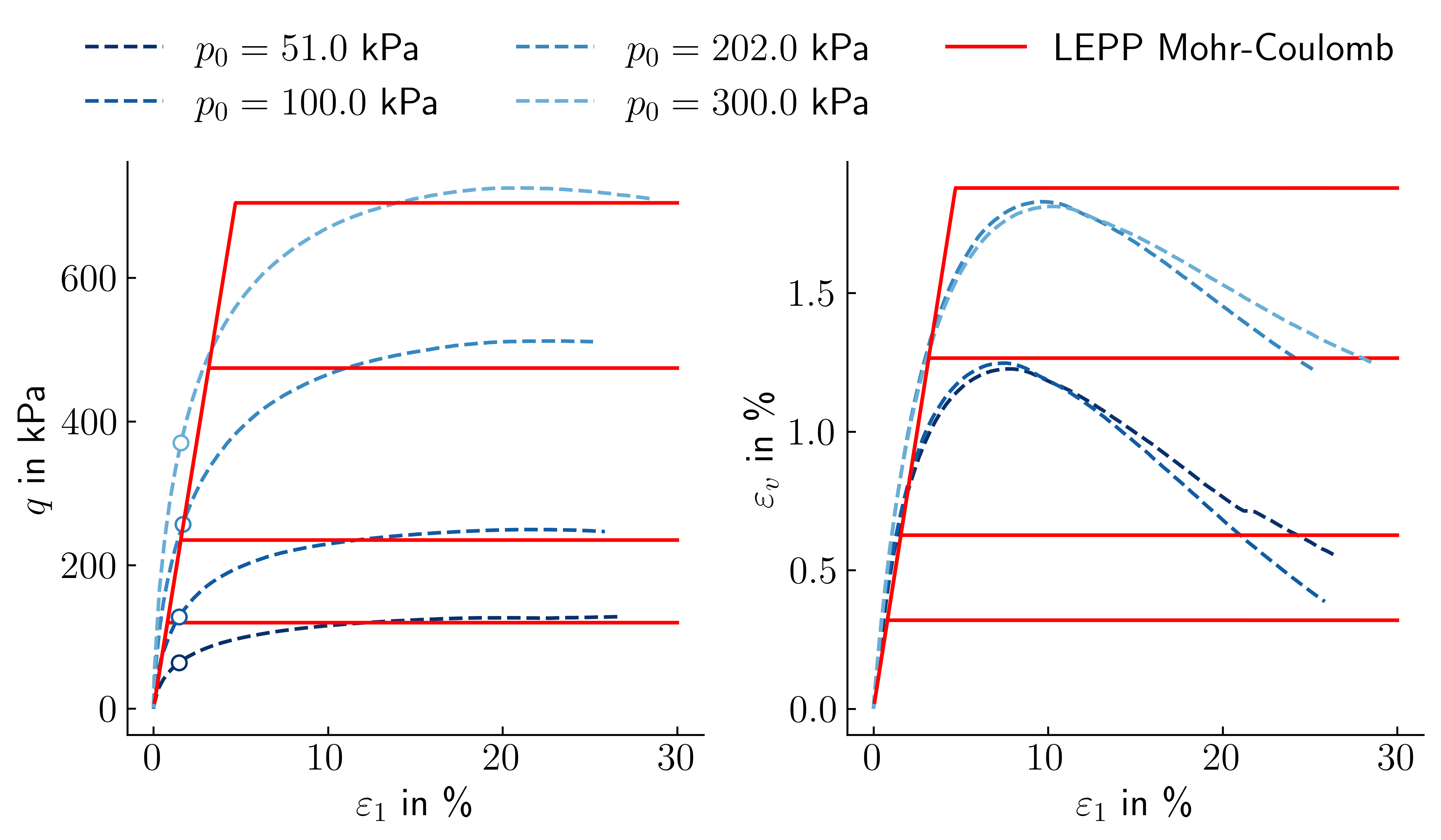
Figure 9. Stress and strain paths of drained triaxial compression tests on Karlsruhe Finesand and corresponding simulations with the LEPP MC model.

From Figure 9 it can be seen that a reasonable agreement between the simulation and the experiment is obtained in terms of maximum deviatoric stress (shear strength). However, it becomes also obvious that deformations observed in the experiment are not well captured by the LEPP MC model. The linear nature of the model does not offer enough flexibility to fit the (1) non-linear deformation characteristics observed in the experiment and (2) the pressure dependence of $E_{50}$. The worst agreement is observed in terms of the development of volumetric strain $\varepsilon_v$.

Disadvantages

One of the main disadvantages of the LEPP MC model is the linear elastic behaviour ($E=const$) until failure. This was already visible in Figure 9, where the nonlinear stress-strain behaviour observed in drained monotonic triaxial tests was not well captured by the model. This shortcoming becomes even more obvious when applying the LEPP MC model to the simulation of oedometric compression tests as shown in Figure 10. The lack of a barotropic stiffness $E(\boldsymbol{\sigma})$ does not allow to capture the observed nonlinear stress-strain behaviour (see also Section stress dependence). Due to this limitation the LEPP MC model should not be used for the prediction of deformations.

Figure 10. Simulation of an oedometric compression test with loading and unloading with the LEPP Mohr-Coulomb model using two different values for the Young's modulus $E=5$ MPa (left) and $E=8$ MPa (right).

In Figures 7 and 8 it was demonstrated that the for $\psi \neq 0$ excessive volumetric deformation might appear under drained conditions. Since no Critical State is considered in the model, no decay of the dilatancy with increasing shear will occur. For undrained conditions this results in a significant overestimation of shear strength due to the development of negative pore water pressures as explained in Section Dilatancy angle

Effects of density (i.e. via the void ratio $e$) are not considered in the LEPP MC model. Different sets of parameters are required to model the behaviour of the same soil (same mineralogical composition, same grain size distribution curve, same grain shape) but at two different densities. This is demonstrated by back-calculating two drained monotonic triaxial tests on Karlsruhe Finesand with identical initial mean effective stress $p_0'$ but different initial void ratios $e_0$. A comparison of the simulation results to the experimental data is given in Figure 11.

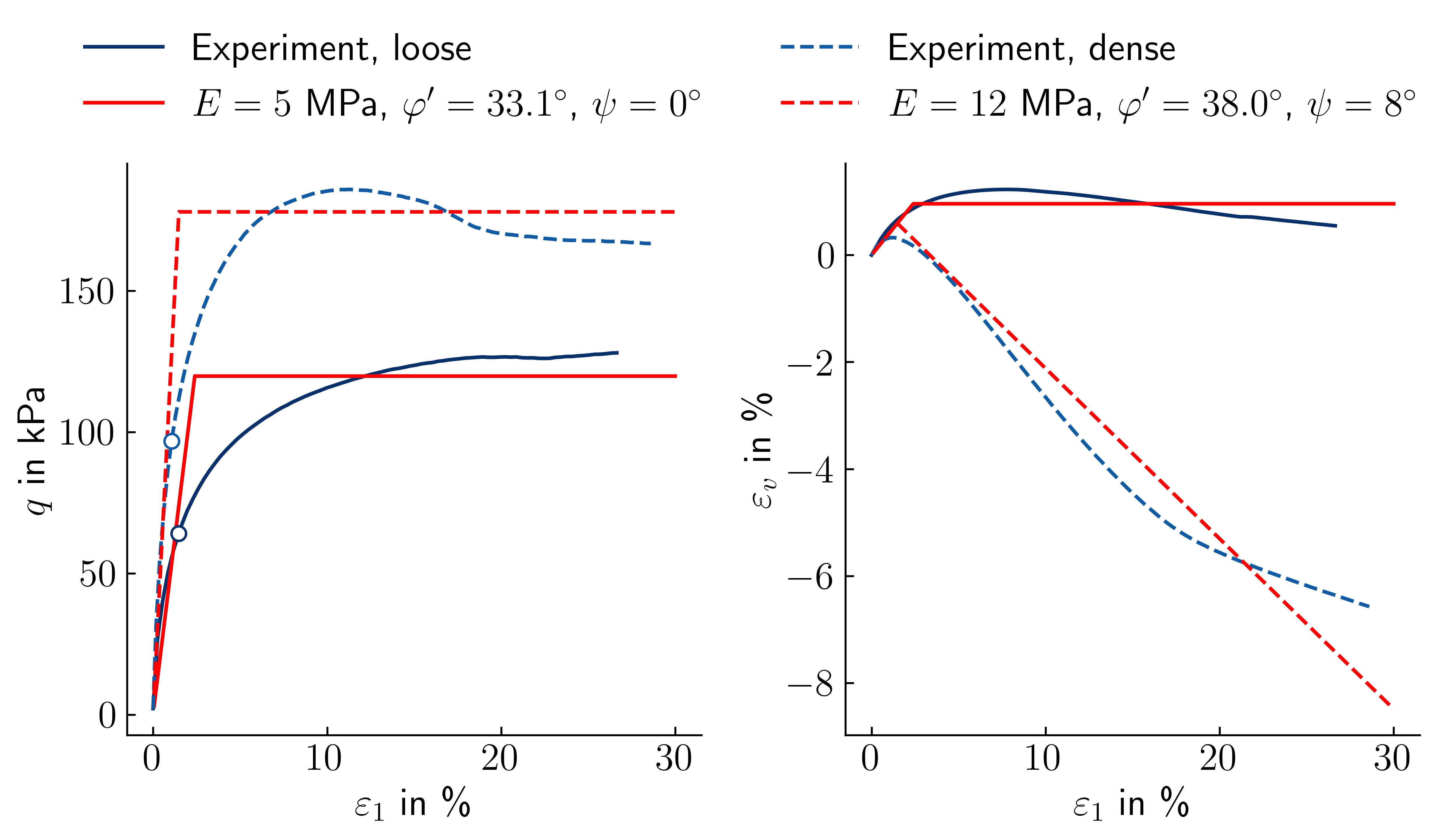
Figure 11. Simulation (red) vs. experimental data (blue) of two drained monotonic triaxial tests on loose and dense Karlsruhe Finesand at $p'_0=51$ kPa.

From the legend of Figure 11 it can be seen that two different sets of parameters are required in order to capture the influence of density on the material behaviour.

P. V. Lade, ‘Modelling the strengths of engineering materials in three dimensions’, Mechanics of Cohesive-frictional Materials, vol. 2, no. 4, pp. 339–356, 1997, doi: https://doi.org/10.1002/ ↩
T. Wichtmann and T. Triantafyllidis, ‘An experimental database for the development, calibration and verification of constitutive models for sand with focus to cyclic loading: part I—tests with monotonic loading and stress cycles’, Acta Geotech., vol. 11, no. 4, pp. 739–761, Aug. 2016, doi: 10.1007/s11440-015-0402-z. ↩