Bio-Cemented hypoplasticity with interganular strain and semifluidized state (BC-Hypo-IGS-SF)
For the validation of the BC-Hypo-IGS-SF implementation available in numgeo, a comparison with the simulation results on Karlsruhe Fine Sand reported in Tafili et al. (2026)1 is made. The BC-Hypo-IGS-SF implementation currently offers access to two different integration schemes:
- Euler–Richardson — explicit scheme with adaptive substepping and error control.
- Forward Euler — explicit scheme with a constant substep size.
Input files
The input files for the benchmark simulations can be downloaded here. The reference results and this manual are kindly written and provided by Hossam Abdellatif and Merita Tafili.
We analyse an undrained cyclic triaxial test with stress amplitude \(q_{\text{ampl}} = 40\ \text{kPa}\).
The initial state is:
- isotropic mean effective stress \(p^\prime_0 = 100\) kPa,
- void ratio \(e_0 = 0.761\),
- intergranular strain \(\boldsymbol{h}_0 = {-0.000080829}\cdot \mathbf{1}\),
- cementation content \(C_c= 0\) %. Following Figures 2-9 include varying \(C_c\).
Cyclic loading is applied using the lab-cyclic-stress-strain-control amplitude, which drives the specimen at strain increments of \(\Delta \varepsilon_{ax}=10^{-6}\).
Notation: \(p^\prime\) denotes mean effective stress, \(q\) the deviatoric stress, and \(\varepsilon_{\text{ax}}\) the axial strain.
Forward Euler (default)
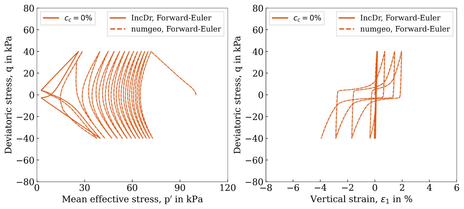
Figure 1: Undrained cyclic triaxial test — comparison of the numgeo implementation (Forward Euler) with the reference solution of Tafili et al. (2026)1.
The agreement between numgeo and the reference solution is excellent in both the \(p'\) – \(q\) and \(\varepsilon_{\text{ax}}\) – \(q\) (with \(\varepsilon_1=\varepsilon_{ax}\)) planes.
In the following, comparisons are presented for oedometric tests, undrained monotonic triaxial tests, and undrained cyclic triaxial tests, demonstrating the excellent agreement between the implementation in numgeo and the reference results reported by Tafili et al. (2026) 1.
Forward Euler
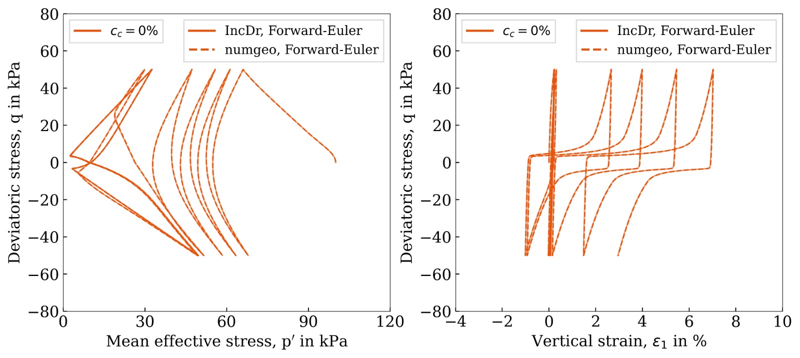
Figure 2: Undrained cyclic triaxial test — comparison of the numgeo implementation (Forward Euler) with the reference solution of Tafili et al. (2026)1.
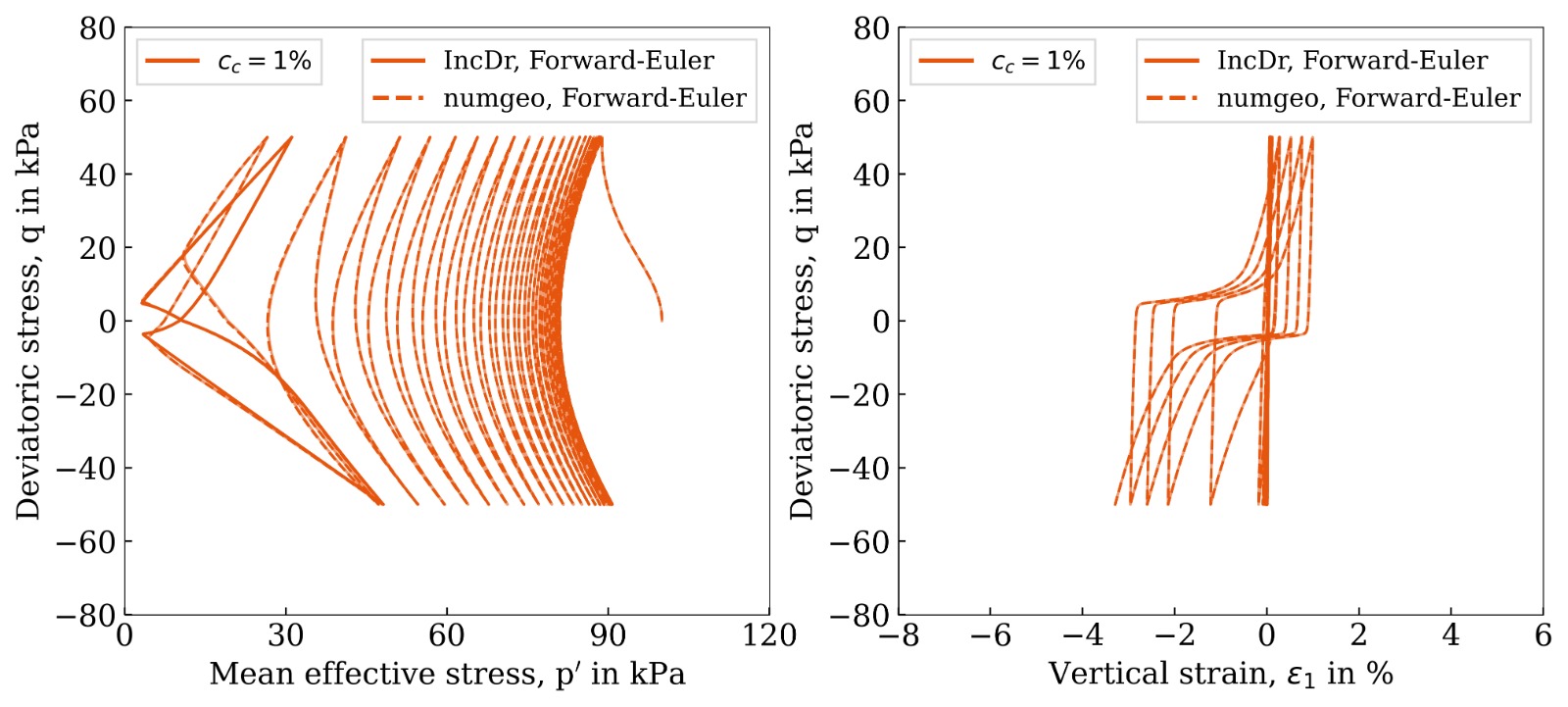
Figure 3: Undrained cyclic triaxial test — comparison of the numgeo implementation (Forward Euler) with the reference solution of Tafili et al. (2026)1.
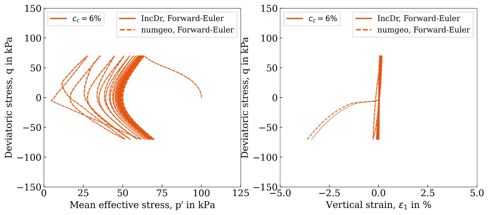
Figure 4: Undrained cyclic triaxial test — comparison of the numgeo implementation (Forward Euler) with the reference solution of Tafili et al. (2026)1.
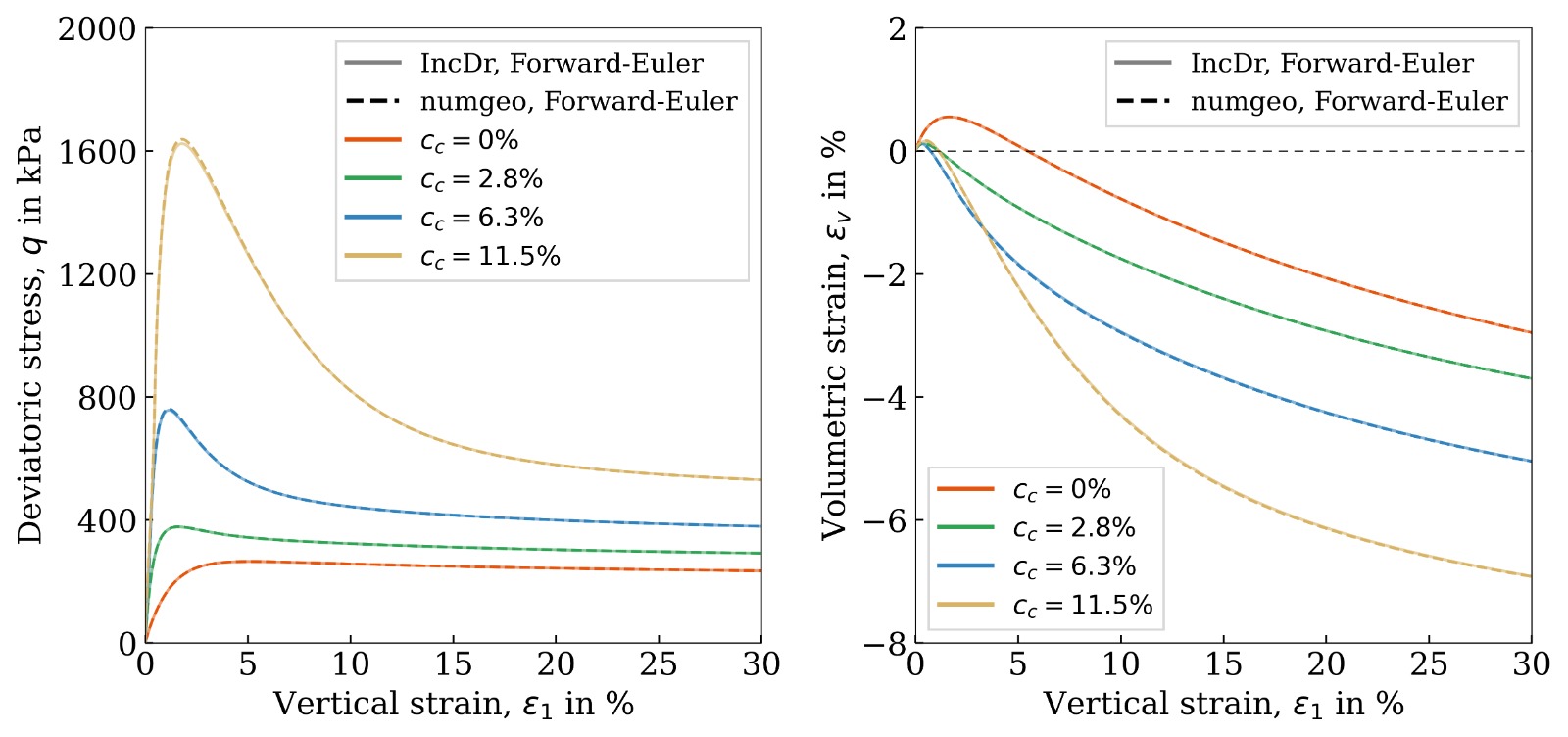
Figure 5: Drained monotonic triaxial tests (\(p_0=100\) kPa, \(D_{r0}\approx\) 60 %) — comparison of the numgeo implementation (Forward Euler) with the reference solution of Tafili et al. (2026)1.
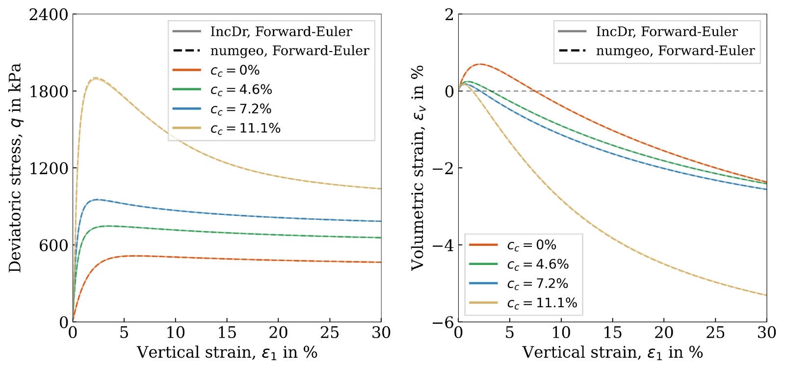
Figure 6: Drained monotonic triaxial tests (\(p_0\) =200 kPa, \(D_{r0}\approx\) 60 %) — comparison of the numgeo implementation (Forward Euler) with the reference solution of Tafili et al. (2026)1.
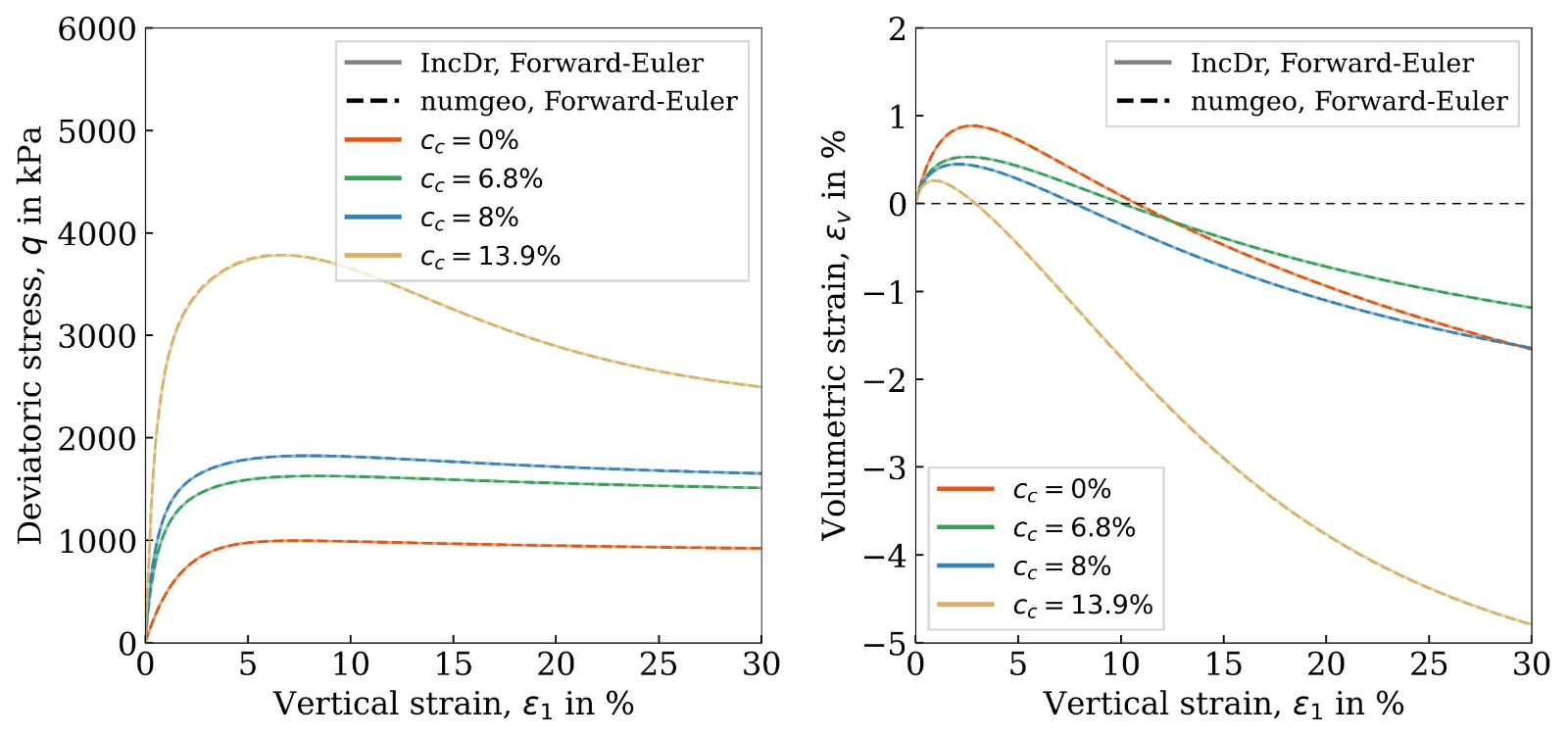
Figure 7: Drained monotonic triaxial tests (\(p_0\) =400 kPa, \(D_{r0}\approx\) 60 %) — comparison of the numgeo implementation (Forward Euler) with the reference solution of Tafili et al. (2026)1.
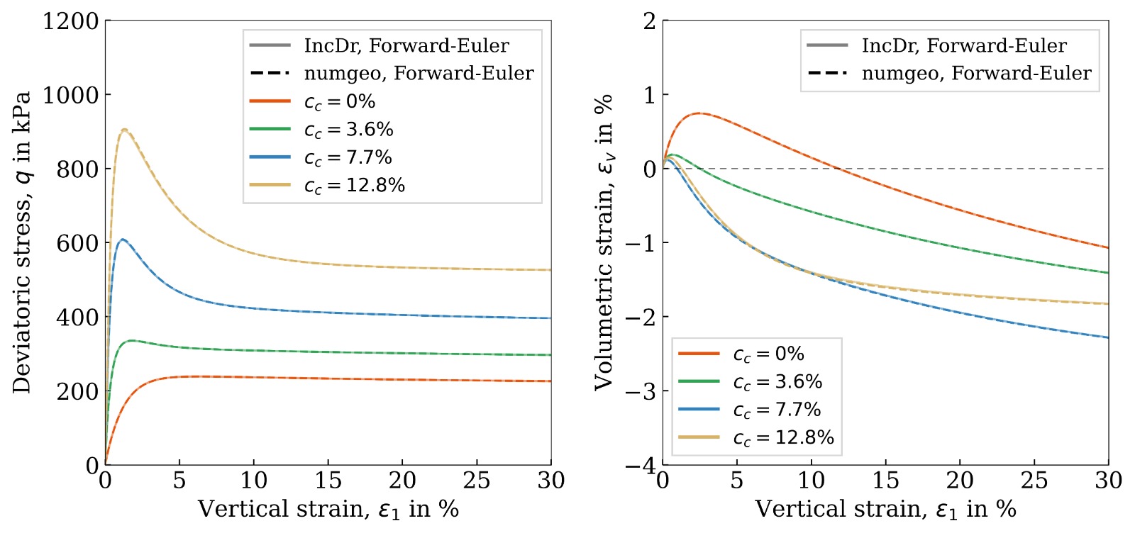
Figure 8: Drained monotonic triaxial tests (\(p_0\) =100 kPa, \(D_{r0}\approx\) 40 %) — comparison of the numgeo implementation (Forward Euler) with the reference solution of Tafili et al. (2026)1.
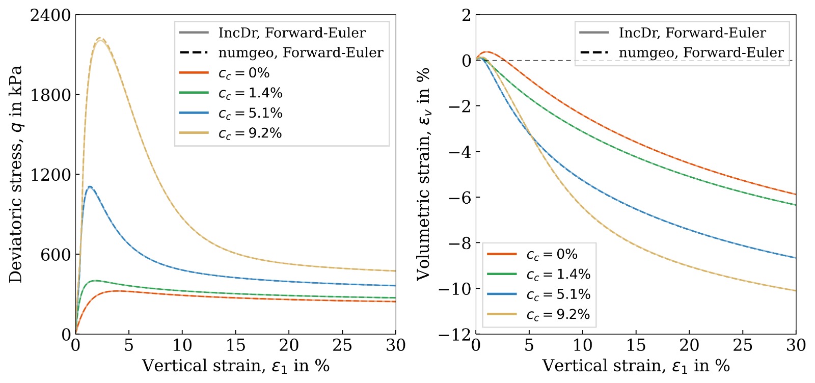
Figure 9: Drained monotonic triaxial tests (\(p_0\) =100 kPa, \(D_{r0}\approx\) 80 %) — comparison of the numgeo implementation (Forward Euler) with the reference solution of Tafili et al. (2026)1.
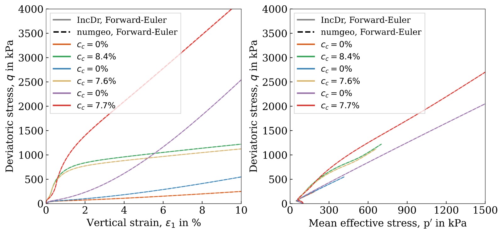
Figure 10: Undrained monotonic triaxial tests (\(p_0\) =100 kPa) — comparison of the numgeo implementation (Forward Euler) with the reference solution of Tafili et al. (2026)1.