Spring-ground-x-tabular: laterally loaded beam on a nonlinear p-y spring bed
This benchmark verifies Spring-ground-x-tabular, including its behaviour once the applied load pushes the response beyond the range covered by the input table. A 2 m long, vertically oriented u2-beam-3D (5 nodes, 4 linear elements, running along the global \(z\)-axis) representing a segment of a large-diameter steel pile is supported along its full length by a bed of Spring-ground-x-tabular springs acting in global \(x\)-direction, with the nonlinear, user-supplied force-displacement law shown in Figure 1 — a typical \(p\)-\(y\)-type lateral soil-reaction curve. Displacement in \(y\) and along the beam axis (\(z\)) is restrained at both ends, and rotation about the beam's own axis (\(r_3\)) is restrained at the base to remove the only otherwise-unconstrained rigid-body mode; the beam is free to move and bend in the loaded (\(x\)) direction along its whole length.
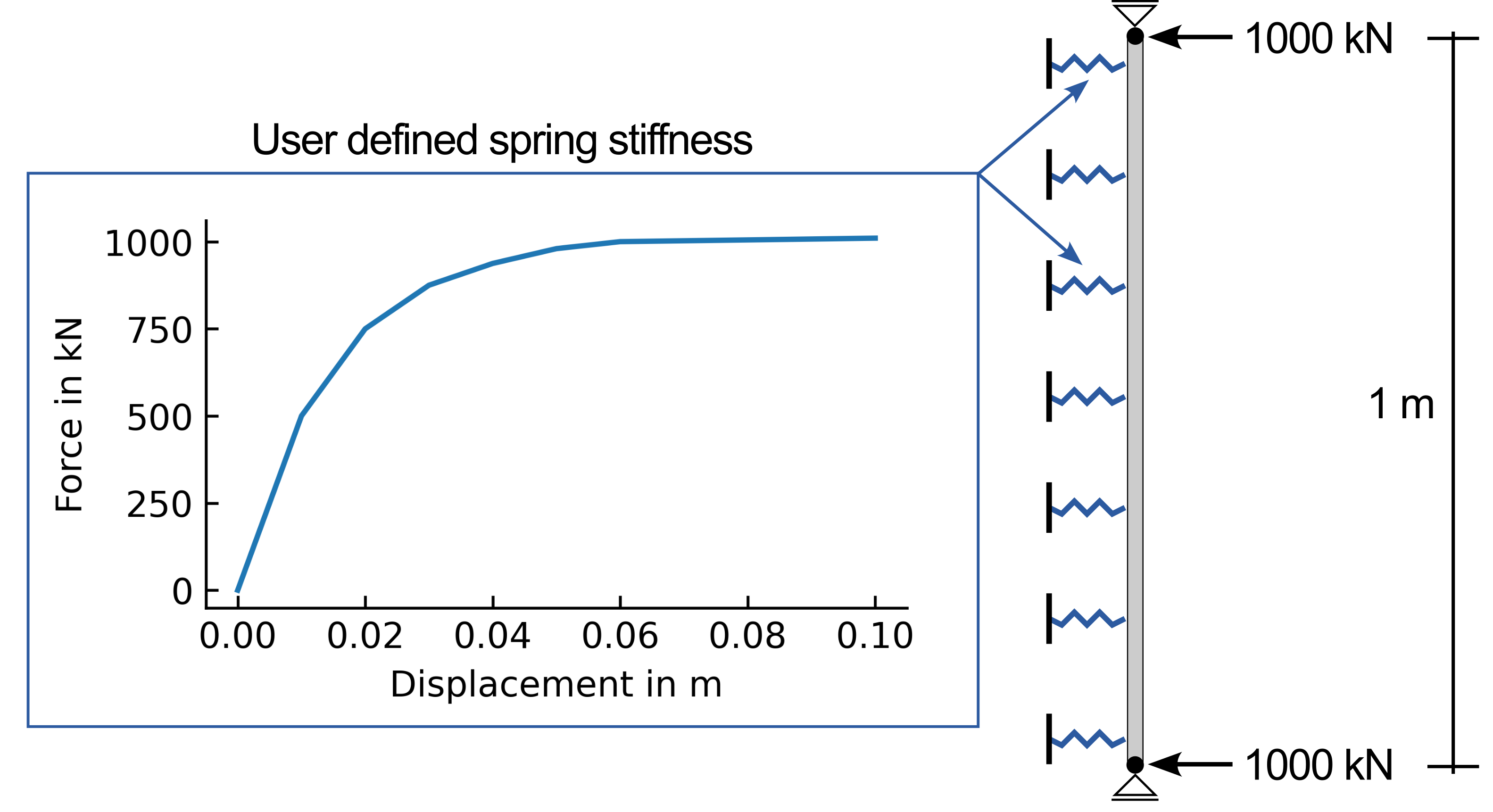
Figure 1: Model setup and the user-defined (\(F\)-\(u\)) spring stiffness (not to scale).
The beam properties (*Beam properties) correspond to a large circular (thin-walled tube) steel cross-section: \(A=2.4819\) m², \(E=210\times10^6\) kPa, \(I_{yy}=I_{zz}=19.3647\) m⁴. Two equal concentrated loads of \(1050\) kN, acting in \(+x\) at both ends of the beam (node sets base and top), are ramped from \(0\) to their full magnitude over the step. Since the beam is very stiff in bending relative to the spring bed over its short length, and the loading is symmetric about the beam's midpoint, the beam deflects essentially as a rigid body — a single lateral displacement \(u\) describes the whole beam to good approximation, and the resisting force of the springs can be calculated as the (tabulated) spring stiffness \(k(u)\) (read from spring-f-u.txt, Figure 1) times the length of the beam (\(L=2\) m).
Input files
Download the input file here
Results
At every instant of the (quasi-static) load ramp, equilibrium requires the total applied load to equal the total spring reaction,
where \(a\in[0,1]\) is the amplitude of the loading ramp. For most of the loading history the required \(k(u)\) stays within the range covered by the table and \(u\) follows directly from the tabulated curve. At \(a=1\) (the end of the step), the required value
exceeds the table's last entry, \(k(0.10~\text{m})=1010\) kN/m — the load was chosen deliberately a bit larger than the table's final value, to demonstrate that the gradient of the last data pair is used once the load exceeds the tabulated data. numgeo continues linearly beyond the last data pair using its gradient,
so that the closed-form displacement at the end of the step is
A comparison of the simulation results (the base node's \(u_1\)) against \(k(u)\cdot L\) evaluated across the loading history — including the final, extrapolated point at \(u=0.26\) m, \(R=2100\) kN — is given in Figure 2. The close agreement, both within the tabulated range and along its linear extrapolation, confirms the correct implementation of the piecewise-linear lookup and its consistent tangent, as well as the extrapolation rule beyond the last table entry.
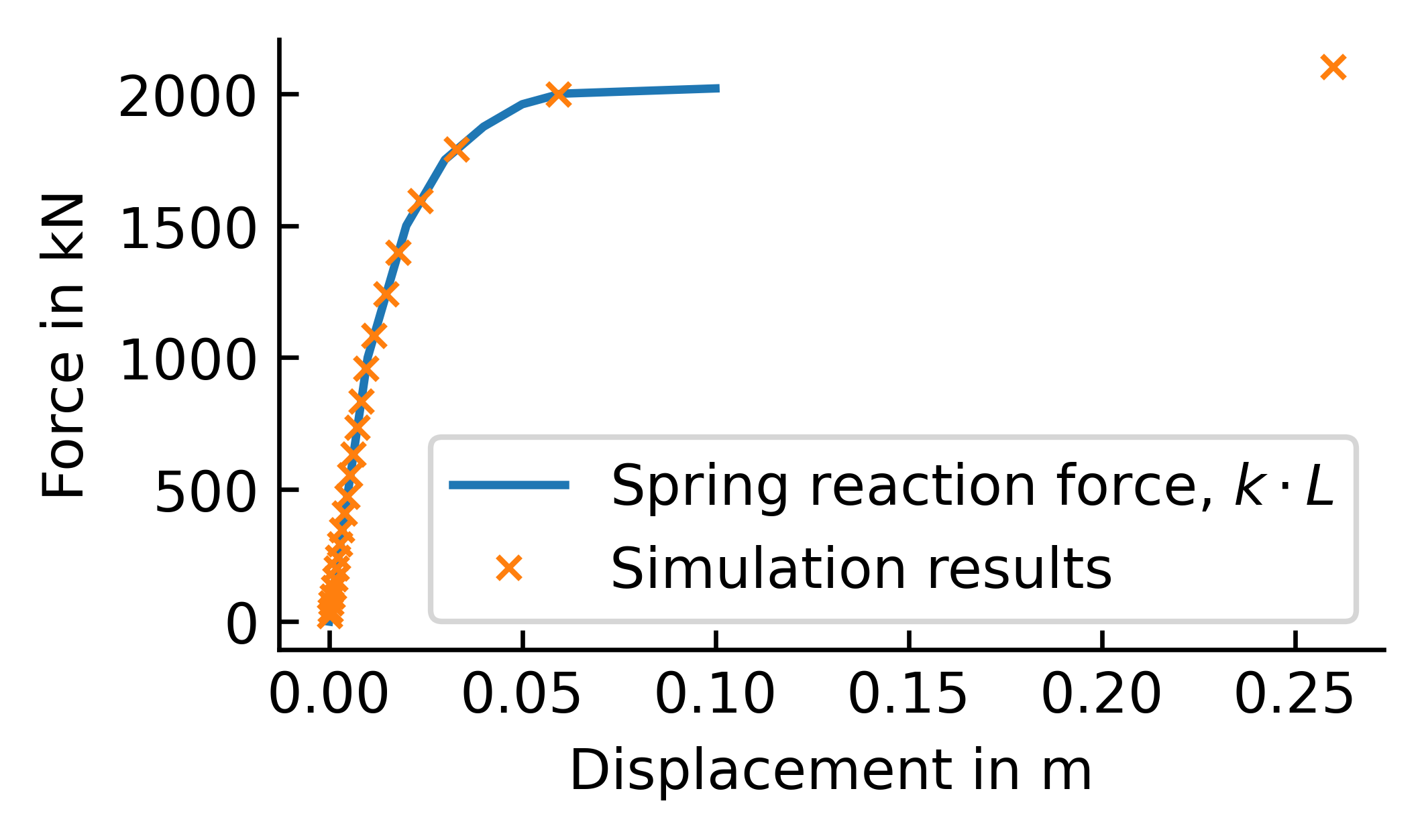
Figure 2: Simulation results vs. \(k(u)\cdot L\) for the laterally loaded beam on a nonlinear spring bed, including the extrapolated point beyond the tabulated range.