Triaxial Test - Consolidated Drained with Unloading and Reloading
Finite Element (FE) representation
The FE representation of the consolidated drained (CD) triaxial test with unloading and reloading cycles follows the same single-element approach as the monotonic CD test. A homogeneous distribution of stress and strain within the sample is enforced by design.
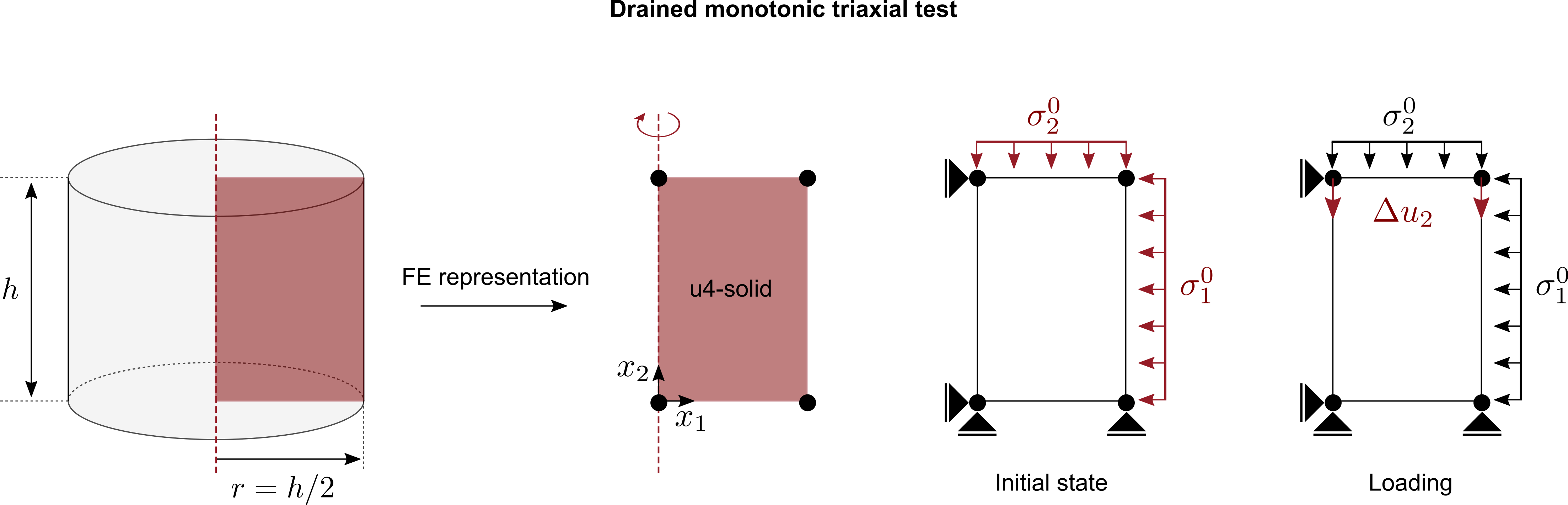
Figure 1. Single-element representation of a drained triaxial compression test
- An axisymmetric solid element with four nodes and linear shape functions for the displacement field is used.
- In the first initial step, the initial conditions are applied: initial stress (\(\sigma_1^0, \sigma_2^0\)), initial void ratio \(e_0\), and any other state variables required by the constitutive model.
- In subsequent loading and unloading steps, the vertical displacement \(u_2\) of the top nodes is prescribed using displacement increments. Rather than specifying a total target displacement for the whole step (as in the monotonic test), here a fixed displacement increment per solver increment is used. This approach, described in more detail below, is particularly suited to unloading-reloading cycles because it allows unloading to be terminated automatically when a target stress state is reached, without needing to know the reversal displacement in advance.
Loading protocol
The simulation consists of five steps after the geostatic initialisation:
| Step | Type | Increments | Displacement per increment | Approximate strain applied |
|---|---|---|---|---|
| Loading-1 | Compression | 200 | \(-0.00025\) m | \(+5\,\%\) |
| Unloading-1 | Extension | up to 200 | \(+0.00025\) m | until \(q = 0\) |
| Loading-2 | Compression | 200 | \(-0.00025\) m | \(+5\,\%\) from current state |
| Unloading-2 | Extension | up to 100 | \(+0.00025\) m | until \(q = 0\) |
| Loading-3 | Compression | 600 | \(-0.00025\) m | \(+15\,\%\) from current state |
The unloading steps are terminated automatically once the axial stress \(\sigma_{22}\) returns to the initial confining pressure of \(-100\,\text{kPa}\), i.e. once the deviatoric stress \(q = \sigma_{22} - \sigma_{11} = 0\).
Key concepts: *Boundary, increment and *Termination
Incremental boundary conditions
In the monotonic CD test, the vertical displacement of the top nodes was prescribed using a linear amplitude ramp:
*Amplitude, name = LoadingRamp, type = ramp
0.0, 0.0, 1.0, 1.0

*Boundary, amplitude = LoadingRamp
ntop, u2, -0.023
Here, the value -0.023 is the total displacement prescribed at the end of the step (when the amplitude reaches 1). This approach requires knowing the final displacement target upfront.
For unloading and reloading cycles this is inconvenient: the displacement at which \(q\) returns to zero (i.e. where unloading should stop) depends on the elastic stiffness of the soil and the current stress state — it is not known beforehand. Instead, we use the increment type boundary condition:
*Boundary, increment
ntop, u2, -0.00025
With type=increment, the specified value is the change in the displacement DOF applied per solver time increment. The displacement accumulates across increments. For a step with fixed time increment size of 1 and a total step time of 200, numgeo will take exactly 200 increments, each advancing \(u_2\) by \(-0.00025\,\text{m}\). The total applied displacement is therefore
which, for a sample of height \(h = 1\,\text{m}\), corresponds to an axial strain of \(\varepsilon_{ax} = 5\,\%\).
Time incrementation
Why fixed time increment sizes? The *Static line for these steps reads:
*Static
1, 200., 1, 1
The four values are: initial increment size, total step time, minimum increment size, maximum increment size. By setting minimum = maximum = 1, the time increment is fixed, numgeo will not try to adapt it. This simplifies the accounting: the number of increments equals the total step time, and the total applied displacement is simply \(N_\text{inc} \times \Delta u\).
See the boundary condition reference for the full documentation of this keyword.
Early termination
Unloading should stop once the deviatoric stress \(q\) has returned to zero, i.e. once the soil is no longer sheared relative to the isotropic stress state. We use the *Termination keyword for this:
*Termination
eall, s22, -100
This instructs numgeo to monitor the stress component \(\sigma_{22}\) (the axial stress) in element set eall after every increment. As soon as \(\sigma_{22}\) reaches \(-100\,\text{kPa}\) — the value of the applied confining pressure — the step is terminated and the simulation continues with the next step. At that point, \(q = \sigma_{22} - \sigma_{11} = -100 - (-100) = 0\,\text{kPa}\), so the sample is unloaded back to an isotropic stress state.
Tip
Without *Termination, we would either have to over-specify the number of unloading increments (risking reversal into tension, which is unphysical for sand) or manually pre-compute the unloading displacement from the elastic stiffness. The termination criterion avoids both problems.
Simulation results
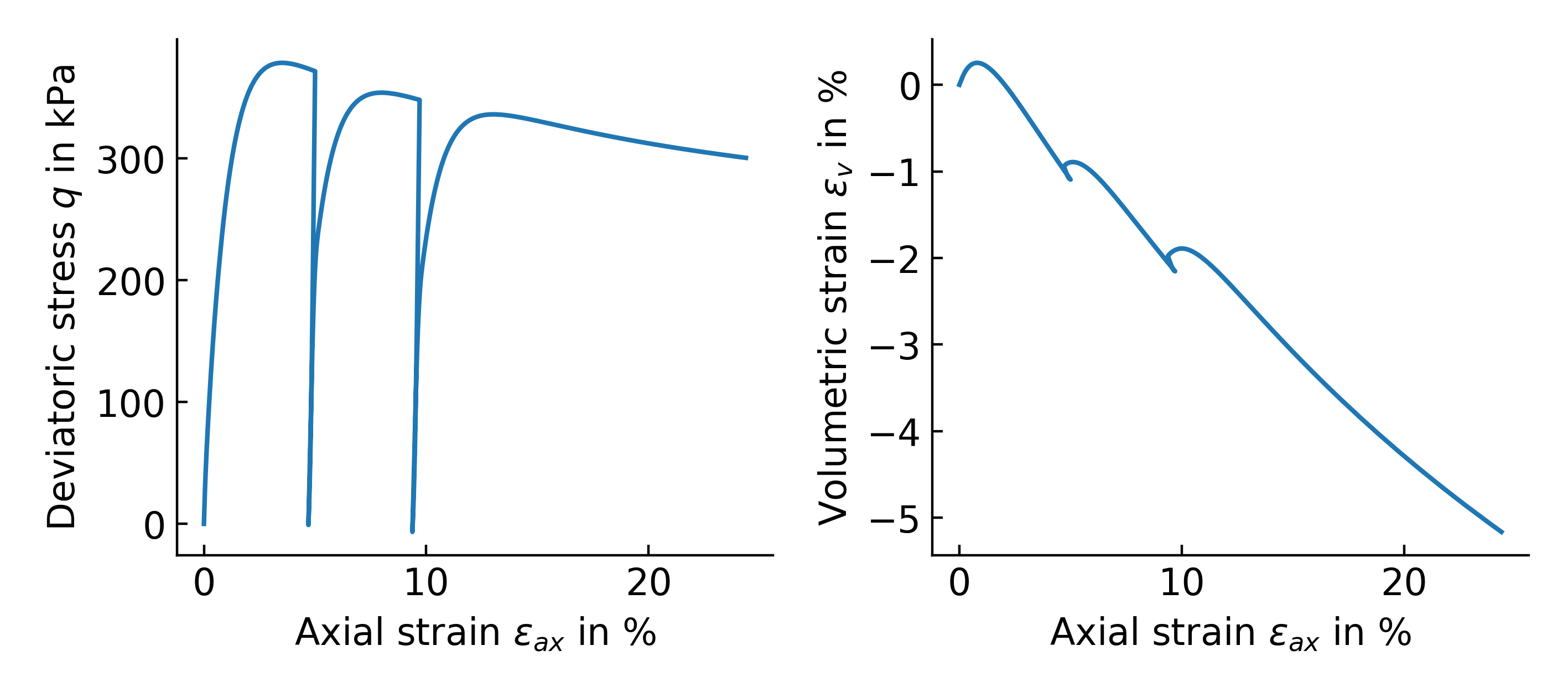
Figure 2. Drained triaxial compression test with unloading and reloading on Karlsruhe Fine Sand (Hypo+ISA): simulation results.
The \(q\)–\(\varepsilon_{ax}\) plot clearly shows the two unloading–reloading loops. After each unloading phase (terminated at \(q = 0\)), the soil is reloaded and follows a stiffer path before eventually rejoining the monotonic backbone curve. The volumetric strain \(\varepsilon_v\)–\(\varepsilon_{ax}\) plot shows the characteristic dilative response of dense sand, with minor changes in slope during the unloading phases reflecting the elastic (recoverable) volumetric response.
Sample numgeo input file
As single-element simulations do not require a complex mesh, the input file is written by hand without a pre-processor.
-
The mesh, element and section definitions are identical to the monotonic CD test. We use an axisymmetric four-node solid element with unit dimensions (\(1\,\text{m} \times 1\,\text{m}\)):
*Node 1 , 0.0 , 0.00 2 , 1.0 , 0.00 3 , 1.0 , 1.0 4 , 0.0 , 1.0 *Nset, Nset=nall 1 , 2 , 3 , 4 *Nset, Nset=nleft 1 , 4 *Nset, Nset=nright 2 , 3 *Nset, Nset=nbottom 1 , 2 *Nset, Nset=ntop 3 , 4 *Element, Type=U4-solid-ax 1 , 1 , 2 , 3 , 4 *Elset, Elset = eall 1 -
Material and section assignment (same as monotonic CD test, using the Hypo+ISA model for Karlsruhe Fine Sand):
*Solid Section, Elset = eall, material=soil *Material, name = soil, phases = 1 *Mechanical = Hypo-ISA 0.578,9958000.0,0.252,0.643,1.066,1.119,0.155,2.906 1.345,0.000179,0.07,10.149,10.832,0.017,762.0,2.078 *Density 1.8 -
Initial conditions. The sample is consolidated isotropically under an effective confining pressure of \(\sigma^0 = 100\,\text{kPa}\). Both horizontal and vertical stresses are therefore equal (\(\sigma_1^0 / \sigma_2^0 = 1\)). The initial void ratio and intergranular strain state are set as for the monotonic CD test:
*Initial conditions, Type = stress, geostatic
eall, 0.0, -100.00, 0.1, -100.00, 1, 1

*Initial conditions, Type = state variables
eall, void_ratio, 0.758169085
eall, int_strain11, -0.0001035
eall, int_strain22, -0.0001035
eall, int_strain33, -0.0001035
eall, int_back_strain11, -5.18e-05
eall, int_back_strain22, -5.18e-05
eall, int_back_strain33, -5.18e-05
Missing *Amplitude definition
No *Amplitude definition is needed in this simulation. Since we are using *Boundary, increment (instead of *Boundary, amplitude=...), the boundary conditions are driven by the per-increment displacement directly and do not require an amplitude function.
-
Geostatic step. The geostatic step initialises the stress field without generating deformations. An isotropic confining pressure of \(100\,\text{kPa}\) is applied on all sides:
*Step, name=Geostatic, inc=1 *Geostatic *Solver, simple *Body force, instant eall, grav, 0.0, 0., -1, 0. *Dload, instant eall, p3, -100 *Dload, instant eall, p2, -100 *Boundary nleft, u1, 0. nbottom, u2, 0. *Output, print *Element output, elset=eall S, E, void_ratio *End Step -
Loading-1. The sample is compressed axially by prescribing a fixed displacement increment of \(\Delta u_2 = -0.00025\,\text{m}\) per time increment. With 200 fixed increments (controlled by
*Static 1, 200., 1, 1), a total axial displacement of \(0.05\,\text{m}\) is applied, corresponding to \(\varepsilon_{ax} = 5\,\%\) for a 1 m sample. The lateral confining pressure is held constant throughout via*Dload:*Step, name = Loading-1, inc = 100000, maxiter = 16 *Static 1, 200., 1, 1 *Solver, simple *Body force, instant eall, grav, 0.0, 0., -1, 0. *Dload, instant eall, p3, -100 *Dload, instant eall, p2, -100 *Boundary, increment ntop, u2, -0.00025 *Boundary nleft, u1, 0. nbottom, u2, 0. *Output, print *Element output, Elset = eall S, E, void_ratio *End Step -
Unloading-1. The sign of the displacement increment is reversed (\(\Delta u_2 = +0.00025\,\text{m}\)) to unload the sample. The step is terminated automatically by the
*Terminationcriterion once \(\sigma_{22}\) returns to \(-100\,\text{kPa}\) (i.e. \(q = 0\)). Up to 200 increments are available, which would correspond to a maximum reversal of \(5\,\%\) — more than sufficient:*Step, name = Unloading-1, inc = 100000, maxiter = 16 *Static 1, 200., 1, 1 *Solver, simple *Body force, instant eall, grav, 0.0, 0., -1, 0. *Dload, instant eall, p3, -100 *Dload, instant eall, p2, -100 *Boundary, increment ntop, u2, 0.00025 *Termination eall, s22, -100 *Boundary nleft, u1, 0. nbottom, u2, 0. *Output, print *Element output, Elset = eall S, E, void_ratio *End Step -
Loading-2. The sample is reloaded from its current unloaded state with the same increment size as Loading-1, applying another \(5\,\%\) axial strain:
*Step, name = Loading-2, inc = 100000, maxiter = 16 *Static 1, 200., 1, 1 *Solver, simple *Body force, instant eall, grav, 0.0, 0., -1, 0. *Dload, instant eall, p3, -100 *Dload, instant eall, p2, -100 *Boundary, increment ntop, u2, -0.00025 *Boundary nleft, u1, 0. nbottom, u2, 0. *Output, print *Element output, Elset = eall S, E, void_ratio *End Step -
Unloading-2. A second unloading phase, this time allowing up to 100 increments (maximum reversal of \(2.5\,\%\)). Again terminated by the
*Terminationcriterion at \(\sigma_{22} = -100\,\text{kPa}\):*Step, name = Unloading-2, inc = 100000, maxiter = 16 *Static 1, 100., 1, 1 *Solver, simple *Body force, instant eall, grav, 0.0, 0., -1, 0. *Dload, instant eall, p3, -100 *Dload, instant eall, p2, -100 *Boundary, increment ntop, u2, 0.00025 *Termination eall, s22, -100 *Boundary nleft, u1, 0. nbottom, u2, 0. *Output, print *Element output, Elset = eall S, E, void_ratio *End Step -
Loading-3. The final loading phase compresses the sample by a further \(15\,\%\) (600 increments × \(0.00025\,\text{m}\) = \(0.15\,\text{m}\)), driving it well into the critical state regime:
*Step, name = Loading-3, inc = 100000, maxiter = 16 *Static 1, 600., 1, 1 *Solver, simple *Body force, instant eall, grav, 0.0, 0., -1, 0. *Dload, instant eall, p3, -100 *Dload, instant eall, p2, -100 *Boundary, increment ntop, u2, -0.00025 *Boundary nleft, u1, 0. nbottom, u2, 0. *Output, print *Element output, Elset = eall S, E, void_ratio *End Step -
The input file is closed with:
*End Input
Evaluation script
The following Python script was used to produce Figure 2 from the print output file written by numgeo:
#%%
import numpy as np
import matplotlib.pyplot as plt
plt.rcParams['xtick.direction'] = 'in'
plt.rcParams['ytick.direction'] = 'in'
plt.rcParams['text.usetex'] = False
plt.rcParams['font.size'] = 12
plt.rcParams['axes.spines.right'] = False
plt.rcParams['axes.spines.top'] = False
def cm2inch(*tupl):
inch = 2.54
if isinstance(tupl[0], tuple):
return tuple(i/inch for i in tupl[0])
else:
return tuple(i/inch for i in tupl)
sim = np.genfromtxt('./sim-print-out/EALL_element_1.dat', skip_header=1)
fig, (ax1,ax2) = plt.subplots(ncols=2, sharey=False, figsize=cm2inch(18,8))
ax1.plot(-sim[:,8]*100, -(sim[:,2]-sim[:,1]), label='Simulation')
ax1.set_ylabel('Deviatoric stress $q$ in kPa')
ax1.set_xlabel('Axial strain $\\varepsilon_{ax}$ in %')
ax2.plot(-sim[:,8]*100, -(sim[:,7]+sim[:,8]+sim[:,9])*100., label='Simulation')
ax2.set_ylabel('Volumetric strain $\\varepsilon_{v}$ in %')
ax2.set_xlabel('Axial strain $\\varepsilon_{ax}$ in %')
fig.tight_layout()
plt.savefig('./triaxCD-unload-reload-sim.png', dpi=400)
plt.show()
The print output file EALL_element_1.dat contains all stress and strain output written during all steps in sequence. numgeo appends output from each step to the same file, so no merging is required for post-processing.
Complete input file
**=~~=~~=~~=~~=~~=~~=~~=~~=~~=~~=~~=~~=~~=~~=~~=~~=~~=~~=~~=~~=~~=~~=~~=~~=~~=
** numgeo-ACT
** Copyright (C) 2022 Jan Machacek
**=~~=~~=~~=~~=~~=~~=~~=~~=~~=~~=~~=~~=~~=~~=~~=~~=~~=~~=~~=~~=~~=~~=~~=~~=~~=
*Node
1 , 0.0 , 0.00
2 , 1.0, 0.00
3 , 1.0, 1.0
4 , 0.0, 1.0
*Nset, Nset=nall
1 , 2 , 3 , 4
*Nset, Nset=nleft
1 , 4
*Nset, Nset=nright
2 , 3
*Nset, Nset=nbottom
1 , 2
*Nset, Nset=ntop
3 , 4
*Element, Type=U4-solid-ax
1 , 1 , 2 , 3 , 4
*Elset, Elset = eall
1
** ----------------------------------------
*Solid Section, Elset = eall, material=soil
** ----------------------------------------
*Material, name = soil, phases = 1
*Mechanical = Hypo-ISA
0.578,9958000.0,0.252,0.643,1.066,1.119,0.155,2.906
1.345,0.000179,0.07,10.149,10.832,0.017,762.0,2.078
*Density
1.8
** ----------------------------------------
*Initial conditions, Type = stress, geostatic
eall, 0.0, -100.00, 0.1, -100.00, 1, 1
*Initial conditions, Type = state variables
eall, void_ratio, 0.758169085
eall, int_strain11, -0.0001035
eall, int_strain22, -0.0001035
eall, int_strain33, -0.0001035
eall, int_back_strain11, -5.18e-05
eall, int_back_strain22, -5.18e-05
eall, int_back_strain33, -5.18e-05
** ----------------------------------------
*Step, name=Geostatic, inc=1
*Geostatic
*Solver, simple
*Body force, instant
eall, grav, 0.0, 0., -1, 0.
*Dload, instant
eall, p3, -100
*Dload, instant
eall, p2, -100
*Boundary
nleft, u1, 0.
nbottom, u2, 0.
*Output, print
*Element output, elset=eall
S, E, void_ratio
*End Step
** ----------------------------------------
*Step, name = Loading-1, inc = 100000, maxiter = 16
*Static
1, 200., 1, 1
*Solver, simple
*Body force, instant
eall, grav, 0.0, 0., -1, 0.
*Dload, instant
eall, p3, -100
*Dload, instant
eall, p2, -100
** The loading is applied as a series of displacement increments
** of size 0.00025 (compression). For the given element height of 1 m
** this results in (axial) strain increments of 0.025% (per displacement increment)
** The number of applied increments depends on the step incrementation.
** To keep things easy, we chose time increments of 1 (s) such that the
** total time * increment size renders directly the final applied displacement/strain
** In the present case: u_tot = 200 * -0.00025 = -0.05 m (or 5% compressive strain)
*Boundary, increment
ntop, u2, -0.00025
*Boundary
nleft, u1, 0.
nbottom, u2, 0.
*Output, print
*Element output, Elset = eall
S, E, void_ratio
*End Step
** ----------------------------------------
*Step, name = Unloading-1, inc = 100000, maxiter = 16
*Static
1, 200., 1, 1
*Solver, simple
*Body force, instant
eall, grav, 0.0, 0., -1, 0.
*Dload, instant
eall, p3, -100
*Dload, instant
eall, p2, -100
** The unloading is modelled analogously to the displacement-controlled
** loading in the previous step. However, the unloading should stop at q=0 kPa.
** Since the strain at which q=0 is reached is unknown a priori, we couple
** the incremental loading with an early termination criterion.
** The step is terminated once the axial stress reaches its initial value of 100 kPa
** again, such that q = s22 - s11 = 0.
*Boundary, increment
ntop, u2, 0.00025
*Termination
eall, s22, -100
*Boundary
nleft, u1, 0.
nbottom, u2, 0.
*Output, print
*Element output, Elset = eall
S, E, void_ratio
*End Step
** ----------------------------------------
*Step, name = Loading-2, inc = 100000, maxiter = 16
*Static
1, 200., 1, 1
*Solver, simple
*Body force, instant
eall, grav, 0.0, 0., -1, 0.
*Dload, instant
eall, p3, -100
*Dload, instant
eall, p2, -100
*Boundary, increment
ntop, u2, -0.00025
*Boundary
nleft, u1, 0.
nbottom, u2, 0.
*Output, print
*Element output, Elset = eall
S, E, void_ratio
*End Step
** ----------------------------------------
*Step, name = Unloading-2, inc = 100000, maxiter = 16
*Static
1, 100., 1, 1
*Solver, simple

*Body force, instant
eall, grav, 0.0, 0., -1, 0.

*Dload, instant
eall, p3, -100
*Dload, instant
eall, p2, -100

*Boundary, increment
ntop, u2, 0.00025

*Termination
eall, s22, -100

*Boundary
nleft, u1, 0.
nbottom, u2, 0.

*Output, print
*Element output, Elset = eall
S, E, void_ratio

*End Step
** ----------------------------------------
*Step, name = Loading-3, inc = 100000, maxiter = 16
*Static
1, 600., 1, 1
*Solver, simple

*Body force, instant
eall, grav, 0.0, 0., -1, 0.

*Dload, instant
eall, p3, -100
*Dload, instant
eall, p2, -100

*Boundary, increment
ntop, u2, -0.00025

*Boundary
nleft, u1, 0.
nbottom, u2, 0.

*Output, print
*Element output, Elset = eall
S, E, void_ratio

*End Step
** ----------------------------------------
*End Input