Ground springs
Ground springs are distributed surface (or beam-line) loads that represent a support of the model by a bed of elastic, Winkler-type springs acting between the finite element mesh and a fixed, immovable ground. They are the natural discretised counterpart of a subgrade-reaction (bedding) modulus: rather than modelling the surrounding soil, rock, or structural support explicitly with additional elements, its stiffness is condensed into a boundary condition acting directly on the surface of interest. Typical applications include the elastic bedding of a raft or a sheet-pile wall, the axial and lateral support of a pile in a Winkler (or nonlinear \(p\)-\(y\)/\(t\)-\(z\)-type) idealisation, or struts and anchors that are installed only during a later stage of the analysis.
Four spring families are implemented, sharing a common structure but differing in how the direction of action is determined and in which elements they attach to — see the Reference Manual for the complete compatibility matrix:
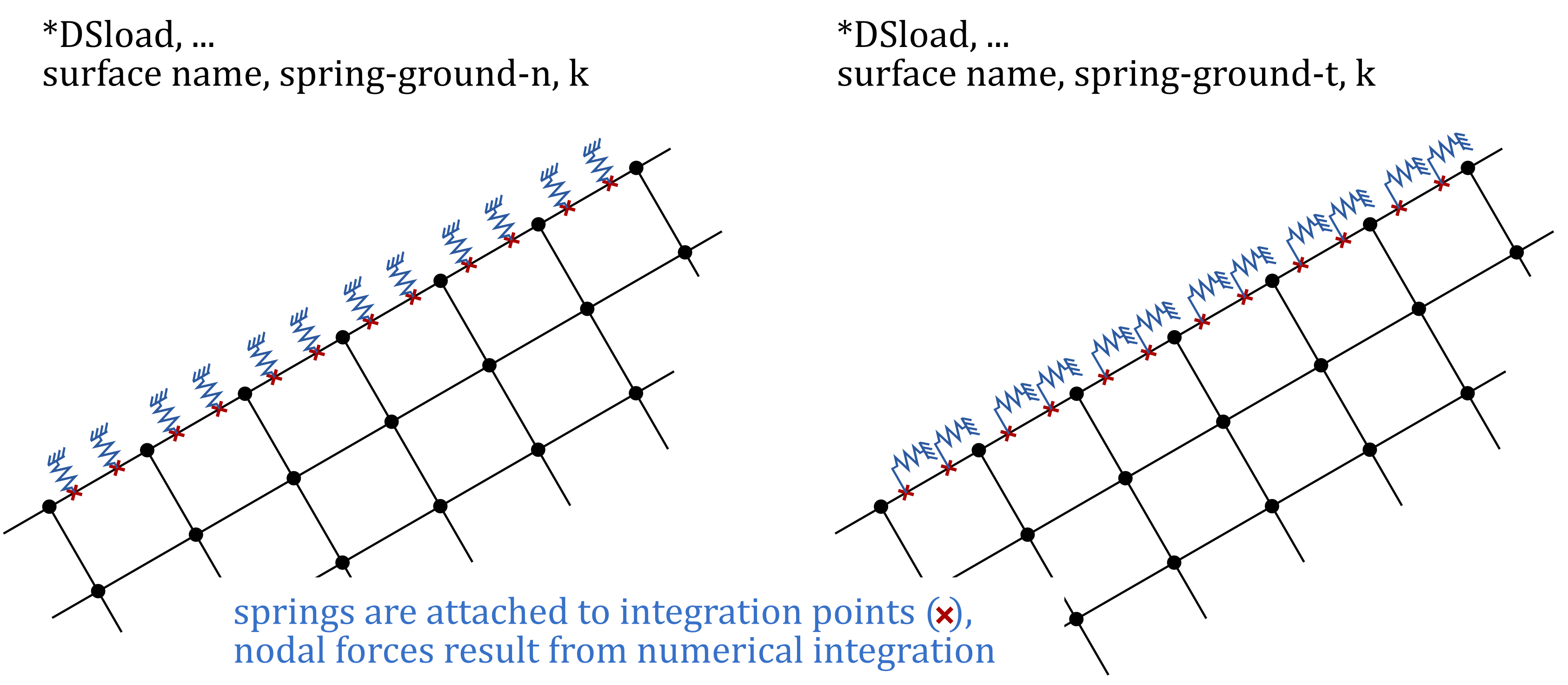
Figure 1: Springs assigned to surfaces using the DSload keyword; the springs are attached at the integration points of the element edges/faces forming the loaded surface.
Constitutive law of the ground spring
At a material point \(\xi\) of the loaded surface (or beam axis) \(\Gamma\), the spring exerts a traction (or, for beam elements, a distributed force per unit length)
i.e. the spring reacts only to the component of the (relative) displacement \(\Delta\boldsymbol{u}\) along its own unit direction of action \(\hat{\boldsymbol{d}}\); the component perpendicular to \(\hat{\boldsymbol{d}}\) produces no traction. \(\tilde k\) is the (possibly nonlinear) stiffness density discussed below, and \(\boldsymbol{u}_{ref}\) is the reference displacement field of the relative displacement formulation, identically zero for the default (total-displacement) formulation.
All four spring families are special cases of this single law, differing only in how \(\hat{\boldsymbol{d}}\) is determined:
| Family | \(\hat{\boldsymbol{d}}\) | Evaluated from |
|---|---|---|
spring-ground-n |
face normal \(\hat{\boldsymbol{n}}\) | reference (undeformed) face geometry |
spring-ground-t |
face tangent \(\hat{\boldsymbol{t}}\) | reference (undeformed) face geometry |
spring-ground-(x,y,z) |
global basis vector \(\hat{\boldsymbol{e}}_i\) | fixed, independent of geometry |
Since \(\hat{\boldsymbol{e}}_i\) is constant, the global-direction springs never require a direction update, not even under nlgeom — only the area (or length) they act over may change with the deformation (see the follower-area term below). The face normal/tangent springs, by contrast, are always evaluated from the reference configuration; there is currently no large-rotation (follower-direction) formulation for them.
Linear and nonlinear (tabular) stiffness
For the constant-stiffness springs, \(\tilde k\) is simply the (constant) value \(k\) supplied in the input file. For the tabular springs (spring-ground-(x,y,z)-tabular), \(\tilde k\) is replaced by a piecewise-linear function \(\tilde k = \tilde k(\Delta u_d)\) read from a two-column \((u,F)\) data file, where \(\Delta u_d := \hat{\boldsymbol{d}}\cdot\Delta\boldsymbol{u}\) is the (scalar) relative displacement along the spring's direction of action:
Both \(F_{\text{table}}\) and \(k_{\text{tan}}\) are obtained from a single table lookup per integration point and iteration; since \(k_\text{tan}\) is exactly the slope of the linear segment that \(F_\text{table}\) is being evaluated on, the resulting tangent is consistent (not just a numerically convenient approximation) and full quadratic Newton convergence is retained across the whole curve, including segments of very different local stiffness (e.g. a near-flat, fully mobilised plateau, Figure 2).
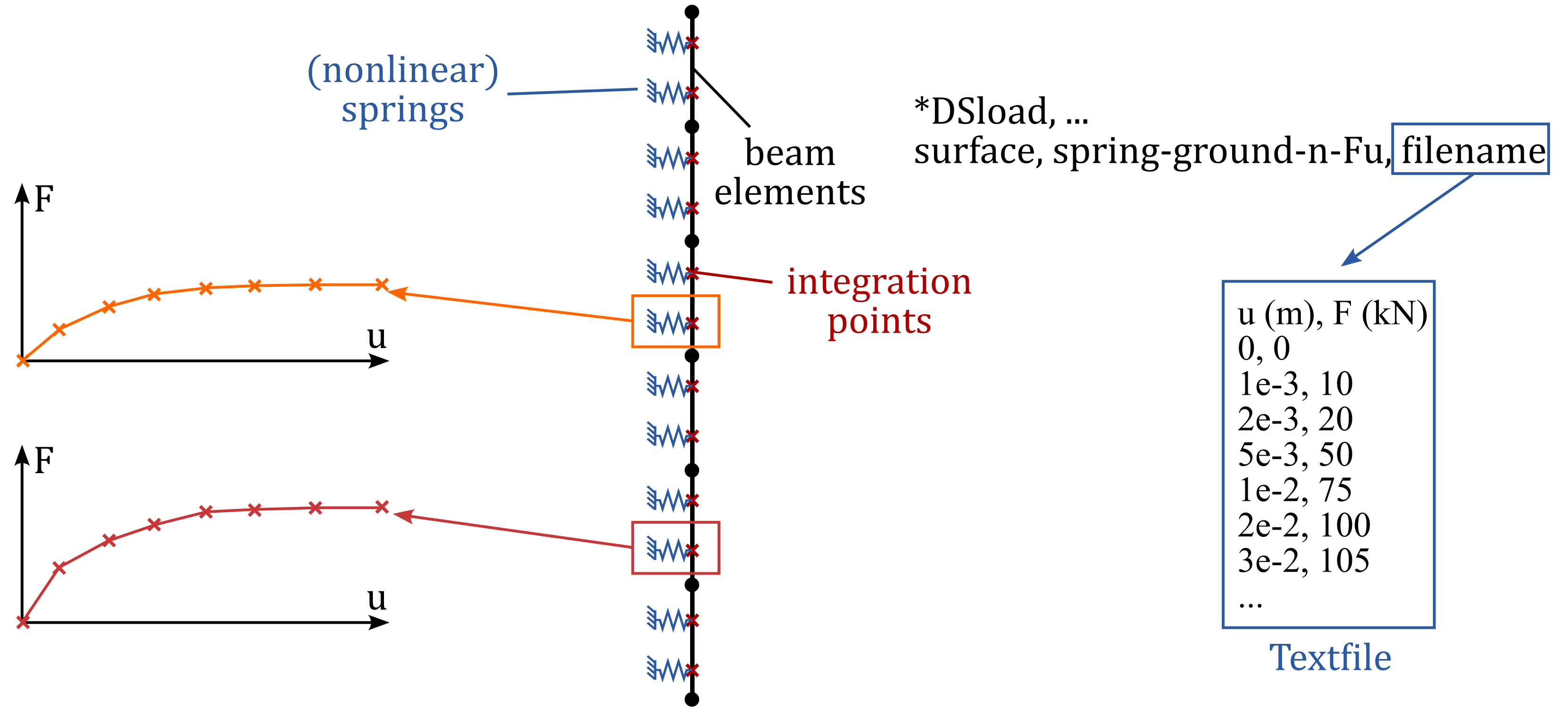
Figure 2: Tabular (nonlinear) spring assigned to a beam element; the piecewise-linear force-displacement law is read from a text file and evaluated (together with its local tangent) at every Gauss point and iteration.
Note that, unlike the constant-stiffness springs, the amplitude mechanism of the enclosing *Dsload statement (instant/ramp/amplitude=...) has no bearing on a tabular spring: there is no externally prescribed magnitude to scale — the entire loading path is generated by the structure's own displacement history through \(F_\text{table}(\Delta u_d)\), exactly as for a physical nonlinear spring.
Discrete contribution
The nodal force vector and its consistent tangent (the contribution to the left-hand-side of the global system) follow from standard Galerkin discretisation of the traction over the loaded geometry \(\Gamma_e\) (an element edge for 2D springs, an element face for 3D springs, or the beam axis for beam springs):
using \(\partial \Delta\boldsymbol{u}/\partial \boldsymbol{u}=\boldsymbol{I}\) (the reference field \(\boldsymbol{u}_{ref}\) is a converged, fixed quantity within a step, see below) and, for the tabular springs, \(\tilde k \to k_{\text{tan}}(\Delta u_d)\). \(f_i\) is assembled into the external force vector with a minus sign (the spring force opposes the displacement) and \(K_{ij}\) is added to the global left-hand-side, consistent with numgeo's convention for solution-dependent loads (e.g. the compliant base or drainage boundary conditions).
What differs between the three element families is the geometric quantity \(\Gamma_e\), its Jacobian \(J_{gp}\), and how \(\hat{\boldsymbol{d}}\) is obtained:
Beam elements (1D)
\(\Gamma_e\) is the beam's own axis; \(J_{gp}=\lVert \mathrm{d}\boldsymbol{X}/\mathrm{d}\xi\rVert\) is the usual arc-length Jacobian, and \(\hat{\boldsymbol{d}}=\hat{\boldsymbol{e}}_i\) (\(i\in\{1,2,3\}\) selected by the X/Y/Z label) is fixed. Linear (2-node) and quadratic (3-node) beam interpolations use 2 and 3 Gauss points, respectively. The translational stride of the beam's degrees of freedom (3 in 2D: \(u_1,u_2,\theta\); 6 in 3D: \(u_1,u_2,u_3,\theta_1,\theta_2,\theta_3\)) is respected when gathering/scattering; the rotational degrees of freedom are not affected by ground springs.
Neither the direction \(\hat{\boldsymbol{d}}\) nor the length Jacobian \(J_{gp}\) is updated under nlgeom for beam springs — the reference-configuration beam length is used regardless of the step's nlgeom setting.
2D solid element edges (N/T)
\(\Gamma_e\) is the element edge to which the load is assigned, treated internally as a 1D sub-element for the purpose of integration (the edge is parametrised exactly like a linear/quadratic beam). \(J_{gp}=\lVert \mathrm{d}\boldsymbol{X}/\mathrm{d}\xi\rVert\cdot 2\pi r\), where the \(2\pi r\) factor is included automatically for axisymmetric elements (\(r\) the radial coordinate of the integration point) and omitted (factor \(1\)) otherwise. \(\hat{\boldsymbol{d}}\) is the face normal \(\hat{\boldsymbol{n}}\) or tangent \(\hat{\boldsymbol{t}}\), computed once from the reference (undeformed) edge geometry — since \(\hat{\boldsymbol{d}}\) does not depend on \(\boldsymbol{u}\), no geometric stiffness term is required for the 2D formulation, even under nlgeom.
3D solid element faces (X/Y/Z)
\(\Gamma_e\) is the element face (a triangle for tetrahedral, a quadrilateral for hexahedral elements) to which the load is assigned. With \(\boldsymbol{a}_1 := \partial\boldsymbol{x}/\partial\xi\), \(\boldsymbol{a}_2 := \partial\boldsymbol{x}/\partial\eta\) the covariant tangent vectors of the parametrised face,
(halved for the triangular parametrisation of a tetrahedral face, matching the standard \(1/2\) weight of a unit triangle). \(\hat{\boldsymbol{d}}=\hat{\boldsymbol{e}}_i\) is fixed, as for beam springs. Under nlgeom, the face geometry is updated with the total displacement, \(\boldsymbol{x}=\boldsymbol{X}+\boldsymbol{u}\), before \(J_s\) is evaluated (an Updated-Lagrangian, "follower area" treatment) — while the constitutive law itself still acts on the relative displacement \(\Delta\boldsymbol{u}=\boldsymbol{u}-\boldsymbol{u}_{ref}\). Under a (default) small-deformation step, \(\boldsymbol{x}=\boldsymbol{X}\) (reference configuration) throughout.
Geometric (follower-area) stiffness, 3D solid faces only
Since \(J_s\) depends on the current nodal positions when nlgeom is active, consistency of \(K_{ij}=\partial f_i/\partial\boldsymbol{u}_j\) requires differentiating \(J_s\) itself, in addition to the material term derived above:
With \(\hat{\boldsymbol{n}} := (\boldsymbol{a}_1\times\boldsymbol{a}_2)/J_s\) the unit face normal, it can be shown (differentiating \(J_s^2 = (\boldsymbol{a}_1\times\boldsymbol{a}_2)\cdot(\boldsymbol{a}_1\times\boldsymbol{a}_2)\) with respect to the position of node \(j\), and using \(\boldsymbol{a}_1,\boldsymbol{a}_2\) linear in the nodal positions through the shape functions) that
so that \(K_{ij}^{\text{geo}} = N_i\,w_{gp}\,\big(\boldsymbol{t}\otimes \boldsymbol{G}_j\big)\), added on top of the material term \(K_{ij}\) above. This geometric contribution is generally unsymmetric — a symmetric solver mode should not be used together with nlgeom ground springs on 3D faces.
Verifying the geometric term
Since a closed-form large-deformation reference solution is rarely available for a full model, the standard (and, for a consistently linearised term, conclusive) way to verify \(\boldsymbol{G}_j\) is to monitor the asymptotic convergence rate of Newton's method in a large-deformation run: an incorrect or missing geometric term degrades convergence from quadratic to linear, or prevents convergence altogether, while a correct one preserves quadratic convergence throughout. See the normal ground-spring benchmark for a worked example.
Relative displacement (installation) formulation
Upcoming release
The relative option will be available with the upcoming release
The default formulation, \(\boldsymbol{u}_{ref}\equiv\boldsymbol{0}\), ties the spring force to the total displacement accumulated since the very beginning of the analysis. For a spring representing a support installed only at some later stage — a strut installed after an excavation step has already deflected the retained wall, for instance — this is physically inappropriate: at the moment of installation the support should be force-free, not already carrying the load corresponding to whatever deformation occurred before it existed.
The relative formulation addresses this by capturing a reference displacement field \(\boldsymbol{u}_{ref}\) once, upon the first assembly of the step in which the spring is (re-)declared:
- If the same spring (matched by load label and surface) was not active in the previous step, \(\boldsymbol{u}_{ref}\) is set to \(\boldsymbol{u}_0\), the converged solution at the end of the previous step — i.e. exactly the state at which the spring is installed. This makes the very first evaluation of the spring force-free, \(\Delta\boldsymbol{u}=\boldsymbol{0}\), regardless of how much deformation had already accumulated elsewhere in the model.
- If the same spring was already active in the previous step, \(\boldsymbol{u}_{ref}\) is instead inherited unchanged from that step, rather than re-captured. Since the inherited field was itself either captured or inherited in a still earlier step, this propagates the original reference state transitively back to the step in which the spring was first activated — the spring is not reset force-free every time it is merely redeclared (e.g. because its magnitude changes) in a subsequent step.
Within a given step, \(\boldsymbol{u}_{ref}\) is treated as a converged, constant field — it is not part of the current iteration's unknowns — so \(\partial \Delta\boldsymbol{u}/\partial\boldsymbol{u} = \partial(\boldsymbol{u}-\boldsymbol{u}_{ref})/\partial \boldsymbol{u} = \boldsymbol{I}\) and the tangent \(K_{ij}\) derived above is entirely unaffected by the choice of formulation; only the residual (force) changes. Combined with a ramp amplitude, the relative formulation produces a smooth, genuinely force-free installation of the support.
Remeshing
\(\boldsymbol{u}_{ref}\) is a snapshot of the global solution vector and is therefore tied to the mesh topology at the moment it was captured. A change of topology (e.g. PFEM remeshing) between capture and use is currently not supported and is caught with a descriptive error rather than silently mapped or discarded.
-
Reference Manual