Embedded beam with implicit interaction surface

*Embedded region, interaction-surface couples a three-dimensional beam to a three-dimensional host continuum through an analytically generated cylindrical shaft surface and, optionally, a disk at a beam end. The interaction surface is implicit: it is neither meshed nor represented by additional surface nodes. Beam and host retain independent degrees of freedom, and their relative motion is evaluated at discrete coupling points on the physical pile circumference and base.

Upcoming release

The *Embedded region, interaction feature will be available with the upcoming release

The formulation belongs to the interaction-surface family introduced by Turello and co-workers and subsequently developed for nonlinear pile–soil interaction and stress recovery Turello et al. (2016, 2017)¹\(^{,~}\)², Granitzer et al. (2024,2026)³\(^{,~}\)⁴\(^{,~}\)⁵. It uses pointwise host interpolation at the physical shaft surface. This differs from the cross-sectionally averaged nonlocal kinematics proposed by Truty ⁶, although both approaches distribute coupling over a finite cross-sectional support.

1. Scope and assumptions

Guest and host elements

The guest set must contain three-dimensional beam elements:

u2-beam-3D;
u3-beam-3D.

Every guest node must provide u1, u2, u3, r1, r2 and r3. Guest and host nodes must be topologically distinct. Coincident coordinates are permitted, but a node shared by a beam and a host continuum element is rejected because the interaction requires independent beam and host translations.

The host set may contain supported three-dimensional tetrahedral or hexahedral continuum elements. Only the three host translations enter the embedded coupling; for coupled displacement–pressure elements, the interaction acts on the solid skeleton.

Kinematic assumptions

The implementation uses the following assumptions:

Coupling-point coordinates, containing host elements and host interpolation coordinates are established in the reference configuration and remain fixed.
The pile cross-section is circular with radius \(R=D/2\).
Beam-side point motion follows the translation and infinitesimal rotation of a rigid cross-section.
Beam and host domains overlap; the physical pile volume is not removed from the host mesh.
The pile is wished in place. Installation-induced changes in stress, density or fabric are not generated automatically.
The interaction is available in implicit analyses. Explicit dynamic steps are rejected.

A coupling point may open and reclose at its fixed point-to-host association. The formulation therefore represents small-sliding contact but is not a finite-sliding surface-to-surface contact algorithm of the type discussed by Wriggers ⁷.

2. Discrete shaft and base geometry

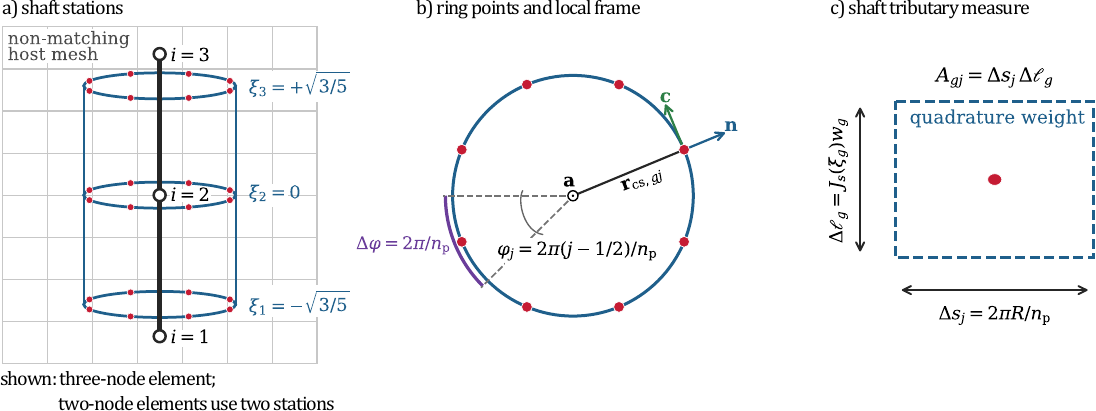
Axial Gauss stations, circumferential coupling points and the tributary shaft measure.

2.1 Shaft quadrature

For a beam element with parent coordinate \(\xi\) and \(n_{\mathrm{bn}}\) nodes, the reference centreline is

\[ \mathbf{x}_{\mathrm a}(\xi)=\sum_{i=1}^{n_{\mathrm{bn}}}N_i(\xi)\mathbf{x}_i, \]

with

\[ \mathbf{x}_{\mathrm a,\xi}(\xi)=\sum_iN_{i,\xi}(\xi)\mathbf{x}_i, \qquad J_{\mathrm s}=\left\|\mathbf{x}_{\mathrm a,\xi}\right\|, \qquad \mathbf a=\frac{\mathbf{x}_{\mathrm a,\xi}}{J_{\mathrm s}}. \]

Two axial Gauss stations are used for a two-node beam and three for a three-node beam. At station \(g\), a deterministic orthonormal frame \((\mathbf e_1,\mathbf e_2,\mathbf a)\) is constructed. The \(j\)th of \(n_{\mathrm p}\) circumferential points is

\[ \varphi_j=\frac{2\pi(j-1/2)}{n_{\mathrm p}}, \]

\[ \mathbf r_{\mathrm{cs},gj} =R\left(\cos\varphi_j\,\mathbf e_1+\sin\varphi_j\,\mathbf e_2\right), \qquad \widetilde{\mathbf x}_{gj}=\mathbf{x}_{\mathrm a}(\xi_g)+\mathbf r_{\mathrm{cs},gj}. \]

The tributary area is

\[ A_{gj}=\frac{2\pi R}{n_{\mathrm p}}J_{\mathrm s}(\xi_g)w_g. \]

For a straight beam, summation over all axial and circumferential points recovers the cylindrical area \(\pi D L\). For a curved three-node beam, the centreline measure is evaluated by Gauss quadrature.

Each coupling point is searched independently in the declared host set. If a point lies outside the host region, it is inactive and its tributary area is not redistributed. A guest element is retained when at least one shaft point is active; an element with no active point is skipped.

2.2 Base-disk quadrature

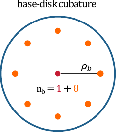
Equal-weight centre-plus-ring cubature used for the base disk.

A declared base node must be an end node of a coupled beam element. The base disk has area \(A_{\mathrm b}=\pi R^2\). Every base point receives the equal weight

\[ A_{\mathrm b,p}=\frac{A_{\mathrm b}}{n_{\mathrm b}}. \]

For \(n_{\mathrm b}>1\), one point lies at the centre and \(n_{\mathrm b}-1\) points lie on a ring of radius

\[ \rho_{\mathrm b}=R\sqrt{\frac{n_{\mathrm b}}{2(n_{\mathrm b}-1)}}. \]

For the default \(n_{\mathrm b}=9\), \(\rho_{\mathrm b}=0.75R\). Provided that all points are active, this rule preserves the disk area, both first area moments, both centroidal second moments and the product moment:

\[ \sum_pA_{\mathrm b,p}=\pi R^2, \qquad \sum_pA_{\mathrm b,p}\mathbf r_p=\mathbf0, \]

\[ \sum_pA_{\mathrm b,p}x_p^2 =\sum_pA_{\mathrm b,p}y_p^2 =\frac{\pi R^4}{4}, \qquad \sum_pA_{\mathrm b,p}x_py_p=0. \]

NB=1 transfers a resultant force only because its lever arm is zero. Inactive base points are omitted without reweighting, so the moment properties above apply only when the complete rule is active.

3. Point kinematics and virtual work

The beam-side displacement of a shaft or base point is

\[ \widetilde{\mathbf u}_{\mathrm p} =\sum_iN_i\left(\mathbf u_i+\boldsymbol\theta_i\times\mathbf r_{\mathrm{cs}}\right), \]

whereas the host-side displacement is

\[ \widetilde{\mathbf u}_{\mathrm h} =\sum_kN_k^{\mathrm h}(\widetilde{\mathbf x})\mathbf u_k^{\mathrm h}. \]

The relative displacement is

\[ \Delta\mathbf u=\widetilde{\mathbf u}_{\mathrm p}-\widetilde{\mathbf u}_{\mathrm h}. \]

At a shaft point, the local basis is

\[ \mathbf Q= \begin{bmatrix} \mathbf a & \mathbf c & \mathbf n \end{bmatrix}, \qquad \mathbf n=\frac{\mathbf r_{\mathrm{cs}}}{R}, \qquad \mathbf c=\mathbf a\times\mathbf n. \]

The relative-displacement components are

\[ \Delta u_{\mathrm a}=\mathbf a\cdot\Delta\mathbf u, \qquad \Delta u_{\mathrm c}=\mathbf c\cdot\Delta\mathbf u, \qquad \Delta u_{\mathrm n}=\mathbf n\cdot\Delta\mathbf u. \]

The cross-section lever arm \(\mathbf r_{\mathrm{cs}}\) is retained in the residual and tangent. An eccentric traction distribution therefore transfers bending and torsional moments in addition to resultant forces.

With local traction

\[ \mathbf t^\ell= \begin{bmatrix} t_{\mathrm a} & t_{\mathrm c} & t_{\mathrm n} \end{bmatrix}^{\mathsf T}, \qquad \mathbf t=\mathbf Q\mathbf t^\ell, \]

the point contribution to virtual work is

\[ \delta W_c=A\,\mathbf t\cdot\delta(\Delta\mathbf u). \]

Beam and host receive equal-and-opposite force contributions. The beam rotational degrees of freedom receive the corresponding moment contribution generated by \(\mathbf r_{\mathrm{cs}}\times\mathbf t\). The same interpolation operators are used in the residual and tangent.

4. Shaft constitutive response

4.1 Unilateral normal contact

Compression is positive. With the default Tension=no,

\[ t_{\mathrm n}=k_{\mathrm n}\langle\Delta u_{\mathrm n}\rangle_+, \]

with algorithmic tangent

\[ D_{\mathrm n}= \begin{cases} k_{\mathrm n}, & \Delta u_{\mathrm n}\ge0,\\ 0, & \Delta u_{\mathrm n}<0. \end{cases} \]

The closed-side tangent is selected at the origin. A negative normal relative displacement denotes opening. At an open point, the complete traction and tangent are suppressed:

\[ \Delta u_{\mathrm n}<0 \quad\Longrightarrow\quad \mathbf t=\mathbf0, \qquad \mathbf D=\mathbf0. \]

The tangential slip reference follows the current tangential motion while the point is open. Recontact therefore starts without a traction jump caused by relative motion accumulated during separation.

Tension=yes activates the bilateral legacy comparison mode. The shaft normal spring then transmits tension and compression, and tangential transfer remains active for either sign of \(\Delta u_{\mathrm n}\).

4.2 Tangential Coulomb-circle slider

At a closed shaft point, define

\[ \mathbf g_{\mathrm t}= \begin{bmatrix} \Delta u_{\mathrm a}\\ \Delta u_{\mathrm c} \end{bmatrix}, \qquad \mathbf s_0= \begin{bmatrix} s_{\mathrm a,0}\\ s_{\mathrm c,0} \end{bmatrix}. \]

The trial traction is

\[ \mathbf t_{\mathrm t}^{\mathrm{tr}} =k_{\mathrm t}(\mathbf g_{\mathrm t}-\mathbf s_0). \]

If \(\|\mathbf t_{\mathrm t}^{\mathrm{tr}}\|\le t_{\mathrm{cap}}\), the point sticks and \(\mathbf D_{\mathrm t}=k_{\mathrm t}\mathbf I_2\). Otherwise, radial return gives

\[ \mathbf m=\frac{\mathbf t_{\mathrm t}^{\mathrm{tr}}} {\|\mathbf t_{\mathrm t}^{\mathrm{tr}}\|}, \qquad \mathbf t_{\mathrm t}=t_{\mathrm{cap}}\mathbf m, \]

\[ \mathbf s=\mathbf g_{\mathrm t}-\frac{\mathbf t_{\mathrm t}}{k_{\mathrm t}}, \]

\[ \mathbf D_{\mathrm t} =\frac{t_{\mathrm{cap}}}{\|\mathbf t_{\mathrm t}^{\mathrm{tr}}\|} k_{\mathrm t}\left(\mathbf I_2-\mathbf m\otimes\mathbf m\right). \]

The axial and circumferential traction components share one circular capacity. The pressure-dependent capacity is evaluated from the last converged state and remains fixed during Newton iterations of the current increment, preserving the return-mapping tangent ⁸.

For Type=Constant, a positive t_ult defines \(t_{\mathrm{cap}}=t_{\mathrm{ult}}\). A non-positive value leaves the tangential shaft response elastic.

For Type=Mohr-Coulomb,

\[ t_{\mathrm{cap}}=\max\left(c+p_{\mathrm{cap}}\tan\varphi,0\right). \]

4.3 Uniform radial ring mode

The implementation retains the pointwise normal operator above. It does not apply a harmonic-mean correction to the uniform radial ring mode. For a closed equal-area ring, the derivative of \(\sum_iA_i\Delta u_{\mathrm n,i}\) has no beam contribution: translational terms cancel around the circumference and \(\mathbf r_i\times\mathbf n_i=\mathbf0\). The uniform mode is therefore carried by host degrees of freedom only. Interface and host stiffnesses act in parallel in the assembled system, not in series. Introducing host compliance once through a harmonic mean and a second time through the resolved host tangent would double-count that compliance.

5. Mechanical traction and capacity pressure

The formulation distinguishes three quantities:

\(t_{\mathrm n}\): mechanical normal traction entering equilibrium;
\(p_{\mathrm{src}}\): non-negative pressure supplied by the selected pressure source;
\(p_{\mathrm{cap}}\): pressure inserted into the Mohr–Coulomb capacity.

If PMAX is specified,

\[ p_{\mathrm{cap}}=\min(p_{\mathrm{src}},p_{\max}); \]

otherwise \(p_{\mathrm{cap}}=p_{\mathrm{src}}\). This cap does not alter mechanical normal traction or contact status and is unrelated to the base limit stress sigma_lim.

5.1 Interface-pressure source

With sigma=Interface, an initial pressure is recovered from the committed host stress during geostatic initialisation,

\[ p_{\mathrm{ini}}=\max(-\mathbf n\cdot\boldsymbol\sigma_0\mathbf n,0). \]

It is recovered with the internally generated inverse-distance map, refreshed while the geostatic step is active and frozen at the first subsequent non-geostatic assembly. Recovery and Lrec apply only to sigma=Soil. At a closed point, the trial source state is

\[ p_{\mathrm{next}}=p_{\mathrm{ini}}+k_{\mathrm n}\Delta u_{\mathrm n}. \]

An open point stores zero pressure. The current increment uses the committed value from the preceding converged increment; the trial value is committed only after convergence. The normal penalty therefore influences both normal compatibility and the pressure available to the Coulomb criterion.

The mechanical normal traction remains \(t_{\mathrm n}=k_n\langle\Delta u_n\rangle_+\) and does not include \(p_{\mathrm{ini}}\). The initial pressure belongs to the shaft-capacity state, not to the equilibrium traction.

5.2 Soil-stress source

With sigma=Soil, the tension-positive committed host stress is recovered at every shaft point and

\[ p_{\mathrm{next}}= \max\left(-\mathbf n\cdot\boldsymbol\sigma^{\mathrm{rec}}\mathbf n,0\right). \]

The current increment again uses the last converged pressure. For supported displacement–pressure hosts, the recovered quantity is the effective stress.

Inverse-distance recovery

Recovery=idw uses admissible integration points in the node-connected patch of the target host element. Its normalised weights are

\[ w_j=\frac{\widehat d_j^{-1}}{\sum_k\widehat d_k^{-1}}, \qquad \widehat d_j=\max\left[d_j,10^{-10}\max(R,h_j)\right]. \]

No integration-volume factor is applied.

Gaussian recovery

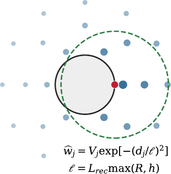
Compact, volume-weighted Gaussian recovery outside the virtual pile volume.

For Recovery=Gaussian,

\[ \ell_{\mathrm{rec}}=L_{\mathrm{rec}}\max(R,h_{\mathrm{tar}}), \qquad h_{\mathrm{tar}}=V_{\mathrm{tar}}^{1/3}, \]

\[ \widehat w_j=V_j\exp\left[-\left(\frac{d_j}{\ell_{\mathrm{rec}}}\right)^2\right], \qquad d_j\le3\ell_{\mathrm{rec}}, \]

\[ w_j=\frac{\widehat w_j}{\sum_k\widehat w_k}. \]

The candidate set is expanded through host-element adjacency and restricted by the compact support. Integration points inside the swept shaft volume are excluded. When ghost=yes, the optional toe half-sphere is excluded as well. If no admissible donor exists, the nearest integration point outside the excluded volume in the complete host region is used and a warning is issued.

The Gaussian procedure is a normalised weighted average, not a superconvergent polynomial patch recovery ⁹. The scale \(\max(R,h_{\mathrm{tar}})\) prevents the support from collapsing when \(R\ll h_{\mathrm{tar}}\), but it does not replace a host-mesh study.

6. Base constitutive response

6.1 Axial mobilisation and history

Let

\[ g_{\mathrm b}=\mathbf a_{\mathrm{out}}\cdot\Delta\mathbf u \]

be the compressive axial relative displacement, and let \(s_{\max,0}\) be the largest converged compressive displacement previously reached. For a monotonic envelope \(\widehat q_{\mathrm b}(s)\),

\[ q_{\mathrm b}= \begin{cases} \widehat q_{\mathrm b}(g_{\mathrm b}), & g_{\mathrm b}\ge s_{\max,0},\\[0.6ex] \widehat q_{\mathrm b}(s_{\max,0})+k_{\mathrm b}(g_{\mathrm b}-s_{\max,0}), & g_{\mathrm b}<s_{\max,0}. \end{cases} \]

Unloading and reloading are therefore linear with slope \(k_{\mathrm b}\) from the previously reached envelope point.

For Baselaw=Elastic-Plastic,

\[ \widehat q_{\mathrm b}(s)= \begin{cases} k_{\mathrm b}s, & \sigma_{\lim}\le0\ \text{or}\ k_{\mathrm b}s\le\sigma_{\lim},\\ \sigma_{\lim}, & k_{\mathrm b}s>\sigma_{\lim}>0. \end{cases} \]

A non-positive sigma_lim therefore gives an elastic axial base response.

For Baselaw=Hyperbolic,

\[ \widehat q_{\mathrm b}(s)= \min\left[ \frac{k_{\mathrm b}s} {\left(1+\left[\dfrac{k_{\mathrm b}s}{f\sigma_{\lim}}\right]^m\right)^{1/m}}, \sigma_{\lim} \right], \]

where Bfac is \(f\ge1\) and Bexp is \(m>0\). The loading tangent before the cap is

\[ k_{\mathrm a}=k_{\mathrm b} \left(1+\left[\frac{k_{\mathrm b}s}{f\sigma_{\lim}}\right]^m\right)^{-(m+1)/m}. \]

For \(f>1\), the nominal capacity is reached at

\[ s^*=\frac{f\sigma_{\lim}}{k_{\mathrm b}} \left(f^m-1\right)^{-1/m}. \]

For \(f=1\), the envelope approaches \(\sigma_{\lim}\) asymptotically. Bexp=1 gives the Kondner hyperbola; increasing \(m\) approaches the elastic–perfectly plastic corner, whereas \(m<1\) gives a more gradual intermediate mobilisation ¹⁰¹¹¹².

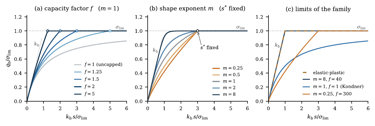
Normalised family of capped generalised-hyperbolic base-mobilisation curves.

The limit is a traction. The corresponding total compressive capacity is

\[ F_{\max}=\sigma_{\lim}\pi R^2. \]

6.2 In-plane sliding and opening

At a closed base point, the in-plane projector and trial traction are

\[ \mathbf P_{\mathrm t}=\mathbf I-\mathbf a_{\mathrm{out}}\otimes\mathbf a_{\mathrm{out}}, \]

\[ \mathbf t_{\mathrm b,t}^{\mathrm{tr}} =k_{\mathrm b}\left(\mathbf P_{\mathrm t}\Delta\mathbf u-\mathbf s_{\mathrm b,t,0}\right). \]

For Type=Constant, a positive t_ult is reused as the in-plane base cap; a non-positive value retains an elastic in-plane response. For Type=Mohr-Coulomb,

\[ t_{\mathrm{cap,b}}=\max(c+q_{\mathrm b}\tan\varphi,0). \]

The in-plane traction is returned radially to this cap. Because the Mohr–Coulomb cap depends on the axial traction, its consistent tangent contains normal-to-tangential coupling and is generally nonsymmetric.

With Tension=no, a tensile axial base trial traction opens the point. Complete base traction and tangent are then zero, and the in-plane slip reference follows the open motion. With Tension=yes, the axial relation remains bilateral and the in-plane spring is linear and uncapped.

7. Elastic ghost zone

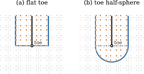
Flat shaft termination (ghost=shaft) and optional toe half-sphere (ghost=yes).

Beam and host occupy overlapping domains. To prevent nonlinear soil response inside the virtual pile volume, selected host integration points may be assigned a linear elastic mechanical response with \(E_{\mathrm{ghost}}\) and \(\nu_{\mathrm{ghost}}\). Their original constitutive state variables remain frozen at the last converged state.

The available geometries are:

ghost=yes: swept shaft cylinder plus a half-sphere of radius \(R\) below every active toe;
ghost=shaft: swept shaft cylinder only;
ghost=no: no constitutive override.

The shaft region follows the actual linear or quadratic beam centreline and does not create spherical caps at the pile head or internal beam-element boundaries. For supported coupled displacement–pressure elements, only the mechanical effective-stress update is replaced; storage, permeability and fluid-coupling terms remain active.

Ghost membership is evaluated at host integration points. The realised elastic volume therefore depends on element size, quadrature and the position of the pile relative to the host mesh. This dependence is particularly strong for one-point reduced-integration elements, for which one classified integration point controls the mechanical response of an entire element. The build reports the number of switched integration points and warns when an active ghost option contains no supported point.

8. Parameter estimates

The interaction stiffnesses have units \(F/L^3\). For an isotropic host, the following mesh-related values provide starting estimates:

\[ k_{\mathrm t}=N_t\frac{G}{R\ln(1+\beta h/R)}, \]

\[ k_{\mathrm n}=N_n\frac{2(1-\nu_i)}{1-2\nu_i}\,k_{\mathrm t}, \]

\[ k_{\mathrm b}=N_b\max\left[ \frac{4G}{(1-\nu_i)\pi R}, \frac{2(1-\nu_i)}{1-2\nu_i}\frac{G}{\beta h} \right]. \]

Here \(h\) is a representative host-element size, \(\beta\) controls the assumed influence range, and \(N_t\), \(N_n\) and \(N_b\) are independent multipliers. These expressions are numerical starting estimates, not universal constitutive parameters. In particular, \(\nu_i\) may be used to control the normal penalty and need not equal the physical soil Poisson ratio. A penalty or stiffness-sensitivity study is required for every new application class. The punch-stiffness term in \(k_{\mathrm b}\) follows the elastic circular-punch solution discussed by Poulos and Davis ¹³.

The interpretation of \(k_{\mathrm n}\) depends on the selected pressure source. With sigma=Soil, it mainly controls normal compatibility. With sigma=Interface, it also affects the pressure available to the shaft-strength criterion.

9. State management and visualisation

Plastic shaft slip, interface-pressure state, axial base history and in-plane base slip are stored as trial and committed values. Every Newton iteration starts from the committed state. Trial values are copied to committed arrays only after convergence, so rejected increments and cutbacks restart from the last accepted interaction state.

The displayed interaction surface is a post-processing reconstruction. One planar quadrilateral is generated for every active shaft coupling point. Its circumferential width is the chord \(2R\sin(\pi/n_{\mathrm p})\), and its axial length is selected so that its area equals the quadrature measure \(A_{gj}\). Cells are centred at beam Gauss stations; adjacent axial bands are therefore separated by small gaps. These spaces do not represent missing interaction area or physical cracks.

The interaction-surface output distinguishes mechanical traction, source pressure, capacity pressure and recovered host normal stress. These quantities should not be interpreted interchangeably.

10. Limitations

The current implementation has the following limitations:

circular sections only;
fixed point-to-host associations in the reference configuration;
no finite-sliding contact search;
no interface dilatancy;
no automatic simulation of installation effects;
no cyclic degradation model;
quadrature-dependent realisation of the ghost volume;
no explicit dynamics;
the same \(k_{\mathrm t}\) is used for axial and circumferential shaft directions;
for Type=Constant, t_ult is reused as the in-plane base cap.

Reference manual

How to use it

References

Diego F. Turello, Federico Pinto, and Pablo J. Sánchez. Embedded beam element with interaction surface for lateral loading of piles. International Journal for Numerical and Analytical Methods in Geomechanics, 40(4):568–582, 2016. doi:10.1002/nag.2416. ↩
Diego F. Turello, Federico Pinto, and Pablo J. Sánchez. Three dimensional elasto-plastic interface for embedded beam elements with interaction surface for the analysis of lateral loading of piles. International Journal for Numerical and Analytical Methods in Geomechanics, 41(6):859–879, 2017. doi:10.1002/nag.2633. ↩
Andreas-Nizar Granitzer, Franz Tschuchnigg, Saman Hosseini, and Sandro Brasile. Insight into numerical characteristics of embedded finite elements for pile-type structures employing an enhanced formulation. International Journal for Numerical and Analytical Methods in Geomechanics, 48(1):223–249, 2024. doi:10.1002/nag.3641. ↩
Andreas-Nizar Granitzer, Franz Tschuchnigg, Haris Felic, Paul Bonnier, and Sandro Brasile. Implementation and appraisal of stress recovery techniques for embedded finite elements with frictional contact. Computers and Geotechnics, 172:106457, 2024. doi:10.1016/j.compgeo.2024.106457. ↩
Andreas-Nizar Granitzer, Saman Hosseini, Tuan Anh Bui, Haris Felic, and Franz Tschuchnigg. Enhanced embedded pile formulation for spatial soil-structure interaction. geotechnik, 49(2):132–145, 2026. doi:10.1002/gete.70034. ↩
Andrzej Truty. Nonlocal fem modeling of piles as beam elements embedded within 3d continuum. Engineering Structures, 277:115460, 2023. doi:10.1016/j.engstruct.2022.115460. ↩
Peter Wriggers. Computational Contact Mechanics. Springer, Berlin, Heidelberg, 2 edition, 2006. doi:10.1007/978-3-540-32609-0. ↩
Juan C. Simo and Robert L. Taylor. Consistent tangent operators for rate-independent elastoplasticity. Computer Methods in Applied Mechanics and Engineering, 48(1):101–118, 1985. doi:10.1016/0045-7825(85)90070-2. ↩
O. C. Zienkiewicz and J. Z. Zhu. The superconvergent patch recovery and a posteriori error estimates. part 1: the recovery technique. International Journal for Numerical Methods in Engineering, 33(7):1331–1364, 1992. doi:10.1002/nme.1620330702. ↩
R. L. Kondner. Hyperbolic stress-strain response: cohesive soils. Journal of the Soil Mechanics and Foundations Division, 89(1):115–143, 1963. doi:10.1061/JSFEAQ.0000479. ↩
J. M. Duncan and C.-Y. Chang. Nonlinear analysis of stress and strain in soils. Journal of the Soil Mechanics and Foundations Division, 96(5):1629–1653, 1970. doi:10.1061/JSFEAQ.0001458. ↩
R. M. Richard and B. J. Abbott. Versatile elastic-plastic stress-strain formula. Journal of the Engineering Mechanics Division, 101(4):511–515, 1975. doi:10.1061/JMCEA3.0002047. ↩
Harry G. Poulos and Edward H. Davis. Pile Foundation Analysis and Design. John Wiley & Sons, New York, 1980. ↩