Embedded anchor pull-out (3D)

This benchmark repeats Embedded anchor pull-out (2D) with a hexahedral host mesh, to verify the host search and shape-function evaluation of *Embedded region, interaction for 3D continuum host elements, and adds a third step verifying the lateral stiffness \(k_n\), which the 2D benchmark does not exercise.

Upcoming release

The *Embedded region, interaction feature will be available with the upcoming release

Model

A soil block of 2.0 m x 1.0 m x 1.0 m is discretised with four U8-SOLID-3D elements. All soil nodes are fully fixed, rendering the host region rigid. A truss (three U2-TRUSS-3D elements, \(EA = 10^6\) kN) extends from \(x = 0.25\) m to \(x = 1.75\) m at \(y = 0.5\) m, \(z = 0.5\) m; the truss nodes deliberately do not coincide with any soil nodes, in \(x\), \(y\), or \(z\). The embedded length, interface stiffnesses and ultimate skin traction are identical to the 2D benchmark:

\[ L = 1.5 \; \mathrm{m} , \qquad k_t = k_n = 100 \; \mathrm{kN/m/m} , \qquad t_{ult} = 10 \; \mathrm{kN/m} . \]

resulting in a pull-out capacity of \(t_{ult} \cdot L = 15\) kN. The tendon attached at the right end of the grout body and is as well idealised as a linear truss element. A schematic of the model is depicted in Figure 1.

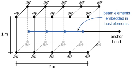
Figure 1: Model setup (not to scale).

Input files

Download the input file here

Steps 1 and 2: axial pull-out (elastic, then plastic)

Identical in setup and result to the 2D benchmark:

\[ u_1(\text{Step 1}) = \frac{F}{k_t \, L} = \frac{7.5}{100 \cdot 1.5} = 0.05 \; \mathrm{m} , \qquad R_1(\text{Step 2}) = t_{ult} \cdot L = 15 \; \mathrm{kN} . \]

Since \(L\), \(k_t\) and \(t_{ult}\) are unchanged and the host is again fully rigid, the 3D result reproduces the 2D one exactly; this confirms that the host element search, the natural-coordinate inversion and the shape-function evaluation are correct for hexahedral host elements (in the 2D benchmark this code path is only exercised for rectangular host elements). A comparison of the simulation results to the analytical solution is provided in Figure 2.

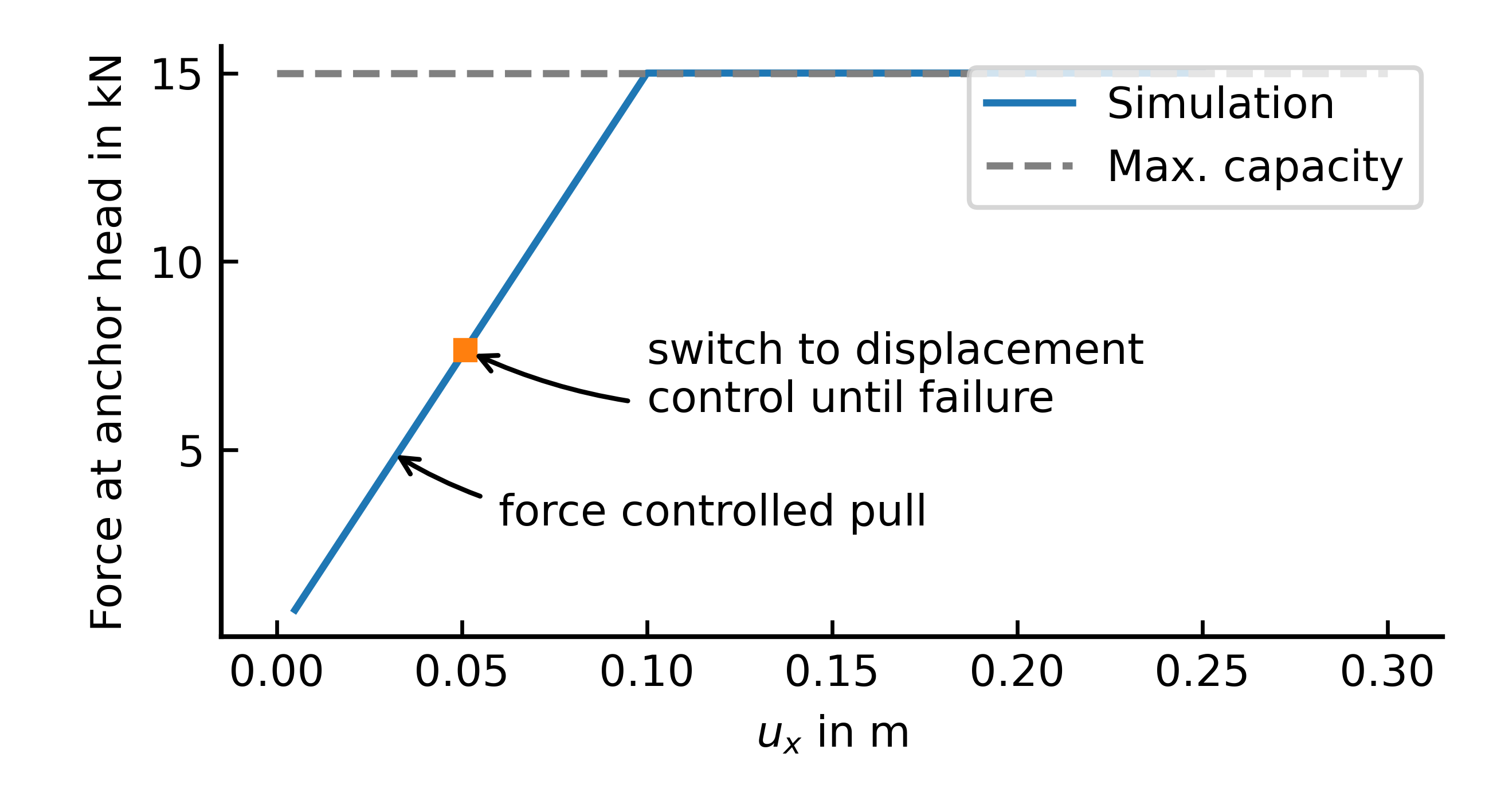
Figure 2: Simulation results vs. analytical solution.

Step 3: lateral stiffness (elastic, displacement controlled)

A uniform lateral displacement \(U_2 = 0.01\) m is prescribed on all four anchor nodes (not only the head), continuing from the end of Step 2. Because the host is rigid and the prescribed displacement is uniform along the embedded length, the relative lateral displacement equals \(0.01\) m everywhere, independent of position:

\[ \Delta u_{\perp}(\xi) = 0.01 \; \mathrm{m} \quad \text{for all } \xi \quad \Rightarrow \quad R_2 = k_n \cdot L \cdot 0.01 = 100 \cdot 1.5 \cdot 0.01 = 1.5 \; \mathrm{kN} , \]

read off as the sum of the \(U_2\) reaction forces over the anchor nodes. Because the axial direction \(\boldsymbol{a}\) is fixed at the (undeformed) reference tangent and the interface modulus \(\boldsymbol{D}\) is diagonal in the \((\boldsymbol{a}, \perp)\) basis, this result is unaffected by the large axial slip already accumulated in Step 2 — Step 3 therefore also confirms the decoupling of the axial and lateral interface response, see Interface law.

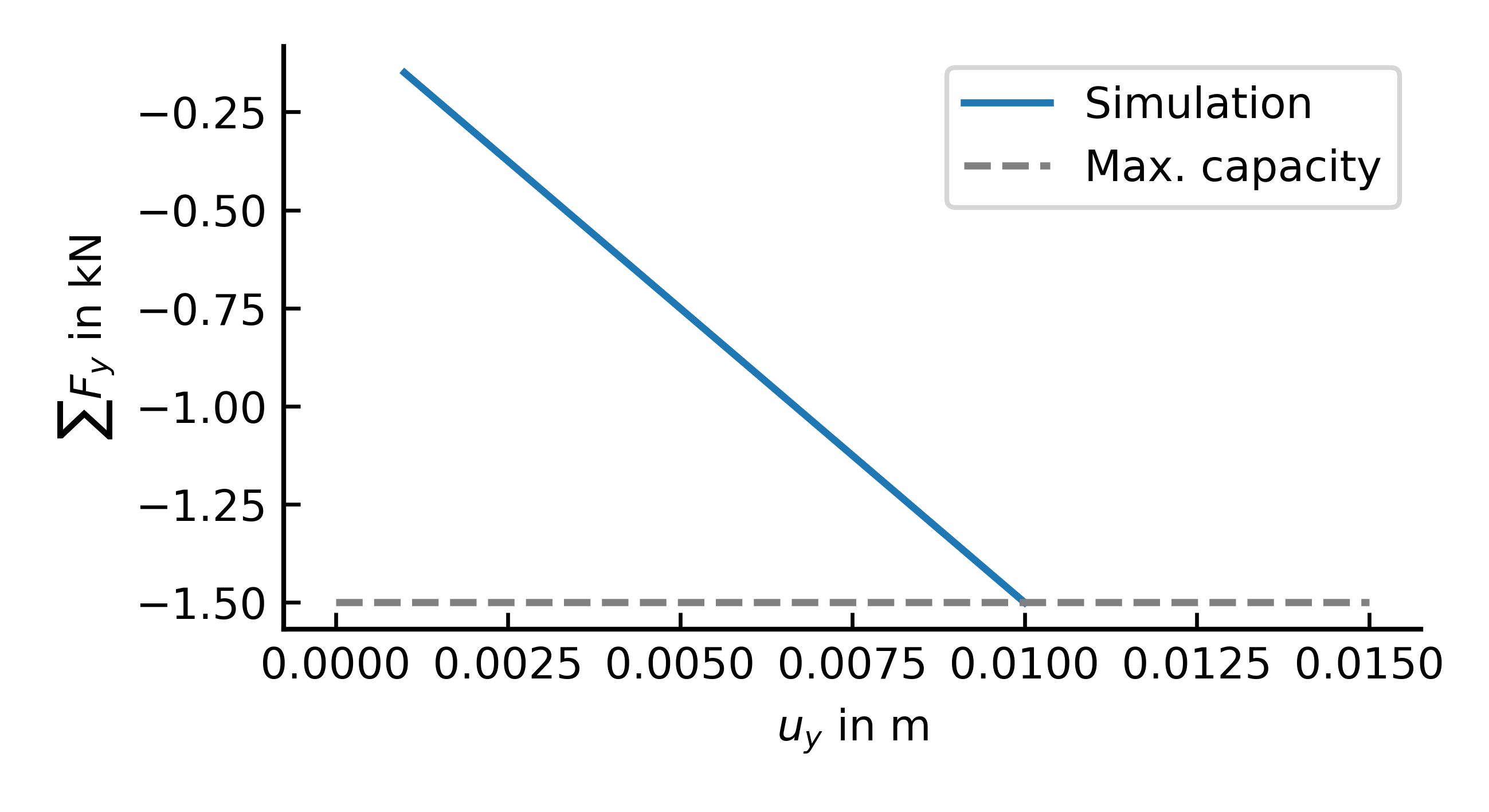
Figure 3: Simulation results vs. analytical solution.